To Notes
IT 403 -- Oct 5, 2016
Review Exercises
- In the Correlation document, look
at the scatterplots of bivariate datasets with various correlations.
- Estimate the correlation r in these situations:
- Height of father, height of son.
i. -0.30 ii. 0.05 iii. 0.70
iv. 0.99 Ans: 0.70
- IQ of husband, IQ of wife.
i. -0.70 ii. 0.00 iii. 0.60
iv. 1.00 Ans: 0.60
- Height of husband, height of wife if men always
married women that were exactly 6 inches shorter.
i. -0.60 ii. 0.60 iii. 0.99
iv. 1.00 Ans: 1.00
- Weight of husband, weight of wife if men always
married women that weighed 70% of their husbands weight.
i. 0.00 ii. 0.50 iii. 0.70
iv. 1.00 Ans: 1.00
- Match the correlation to the dataset:
- GPA in freshman year, GPA in sophomore year. Ans: 0.70
- GPA in freshman year, GPA in senior year. Ans: 0.30
- Length and weight of 2 by 4 boards. Ans: 0.99
-0.50 0.005 0.30 0.70 0.99
- What would happen to the correlation r if
- x were replaced by x + 10.
- y were replaced by 2 times y + 8.
- x and y were interchanged.
Ans: in all three cases, the correlation would remain the same.
- How large must r be to be considered meaningful?
Ans: See the table in the
Correlation document.
- Why is the computed value of r the same whether the SD or the SD+
is used for the x and y standard deviations?
- Use SPSS to compute the pairwise correlations of the variables in the
Nielsen Dataset. The rows
of this dataset are the ratings for various television shows.
Interpret the correlations.
- What is a bivariate normal dataset? Which statistics parsimoniously describe
a bivariate normal dataset?
Ans: x y
SDx SDy rxy.
- How many statistics would you need to parsimoniously describe a
multivariate normal dataset with three variables x, y, and z?
a multivariate normal dataset with k variables?
Ans: For three variables: three sample means, three sample SDs, three sample correlations
rxy, rxz, ryz: 9 total summary statistics.
For k variables: k sample means, k SDs, k(k-1)/2 sample correlations: (k2 + 3k) / 2
total summary statistics.
- Compute the correlation r of this dataset "by hand" using SPSS but not using
Analyze >> Correlate >> Bivariate. If you use SD+ for x and y, don't
forget the correction factor n / (n - 1). Check your answer with Analyze >>
Correlate >> Bivariate.
Ans: r = 0.8.
Linear Correlation
- With the Bears Roster 1985 Dataset, use SPSS to:
- Compute the height in meters and the weight in kilos of the Bears
players. The conversion rates are 0.3048 meters per foot and 0.453592 kilos per pound.
- Use SPSS to create a scatter plot of weight (y-axis) vs. height (x-axis).
- Find the simple linear regression equation for predicting weight in kilos from height in meters.
- Create the residual plot, which is the residuals (y-axis) vs. the predicted values (x-axis).
- For the residual plot, SPSS plots the standardized residuals (ZRESID) vs. the standardized
predicted values (ZPRED).
Project 3
- Look at the project descriptions for Project 3 .
The Regression Fallacy
- During their flight training, Air Force pilots
make two practice landings with their instructor. The pilots that
make a good first landing tend to do worse on the second landing; the
pilots that make a poor first landing do better on the second landing.
Conclusion: criticism helps the pilots, whereas praise hurts them.
Policy change: the supervisor of the flight instructors tells them
to criticise all landings, good or bad. Is this policy change warrented?
- In fact, the criticism is not warrented. This is an example of the
regression fallacy.
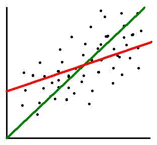
- Look at this graph of pre-test and post-test scores marked by the dots:

The green line indicates where the dots would be if the pre and post scores
were the same. The red line is the regression line, which shows where the
pre-test score and its associated predicted post-test score would lie.
As in the previous example of the Air Force pilots, a student with a high
pre-test score is predicted to do worse on the post-test; a student with
a low pre-test score is predicted to do better on the post-test.
- Practice Problem Collect the following data for adult men:
the subject's height, the height of the subject's father.
- Would you expect a person with a very tall father to be shorter or
taller than his father?
Ans: A very tall person is expected to be shorter than his father
(regression fallacy).
- Would you expect a person with a very short father to be shorter or
taller than his father?
Ans: A very short person is expected to be taller than his father
(regression fallacy).
Additional Regression Problem
- Root Mean Square Error
- A law school finds this relationship between LSAT scores (independent
variable x) and first-year scores (dependent variable y). The data are
bivariate normal. Here are the summary variables:
x = 162 SDx = 6
y = 68 SDy = 10
r = 0.6
- About what percentage of the students have first-year scores over 75?
Because the data are bivariate normal, the first-year scores are
normally distributed, so you can use the normal table.
- Of those students who scored 165 on the LSAT, about what percentage
have first-year scores over 75? Visualize these scores as lying in a thin
vertical rectangle centered at LSAT = 165.
Probability
- The probability that an event occurs is a value between
0 and 1 that indicates how likely that event is to occur;
0 means that the event is impossible, 1 means that the event
is certain to occur.
- The sample space is the set of all possible outcomes
in a probability situation.
- Example 1: Flip a coin once. The sample space is
{head, tail}.
- Example 2: Roll a die once. The sample space is
{1, 2, 3, 4, 5, 6}.
- Example 3: An urn contains 3 red balls and 4 green balls.
Choose a random ball from the urn. The sample space is
{red, red, red, green, green, green, green}.
- Example 4: Choose a random part on an assembly line
and test it. The sample space is {defective, nondefective}.
- Three common ways of determining probabilities:
- Theoretical or A Priori Probability
Assume that all outcomes are equally likely. Suppose you are interested
in the probability that the event A occurs.
P(A) = # ways A can occur / Total # of events
Example 5: What is the probability of getting one head
out of two coin flips?
Sample space S = {HH, HT, TH, TT}
A = Event of getting exactly one head = {HT, TH}
P(A) = # of events in A / # events in S = 2 / 4 = 0.5
- Empirical Probability
Perform an experiment, repeated a large number of times.
Count the number of times s the event
A occurs and the total number of times n the experiment is repeated.
P(A) = s / n
Example 5: Flip a coin 1 million times. 499,523 heads were obtained.
The probability of obtaining a head is 499,523 / 1,000,000 = 0.499523.
- Subjective Probability
Each person uses personal intuition or judgement.
What is the probability that I will need an umbrella today?
Las Vegas oddsmakers combine subjective probabilities
for many sources when determining betting odds.
Example 6: What is the probability that the Bears will win the
Super Bowl in 2012?
A subjective probability can be defined as a fair bet, that is
a bet for which you would be willing to take either side.
- No matter how probabilities are chosen,
a probability distribution is a table that assigns
a probability to each outcome in the sample space:
| Probability Distribution |
| Outcome | Probability |
| HHH | 0.125 |
| HHT | 0.125 |
| HTH | 0.125 |
| THH | 0.125 |
| TTH | 0.125 |
| THT | 0.125 |
| TTH | 0.125 |
| TTT | 0.125 |
When flipping 3 coins, what is the probability of obtaining 1 head?
Ans: There are three ways in the sample space of obtaining one head:
HTT, THT, TTH. Therefore the probability of obtaining one head is
0.125 + 0.125 + 0.125 = 0.375.
- Rules for Probabilities:
- Each probability is between 0 and 1, inclusive.
- The sum of all probabilities of events in the sample space is 1.
- If p is the probability that the event A occurs, then
1 - p is the probability that A does not occur.
Random Variables
We will discuss random variables next time on Oct 12.
- A random variable is a function from the sample space to the set of real numbers.
- Example 7: Pick a person at random. That person's
height is a random variable.
- Example 8: The random variable x is the number of heads
obtained out of two coin flips.
| x |
Probability |
| 0 | 0.25 |
| 1 | 0.50 |
| 2 | 0.25 |
- Example 9: The random variable x is the number of heads
obtained out of three coin flips.
| x |
Probability |
| 0 | 0.125 |
| 1 | 0.375 |
| 2 | 0.375 |
| 3 | 0.125 |
- A random variable that has only two outcomes 0 and 1 is called
a Bernoulli random variable; 1 denotes success and
0 denotes failure. Here is the probability table for a Bernoulli
random variable:
| x |
Probability |
| 0 | 1 - p |
| 1 | p |
- Some examples of Bernoulli random variables:
flipping a coin (T = 0, H = 1), rolling an ace with a single die
(non-ace = 0, ace), shooting a basketball free throw (failure = 0, success = 1),
choosing a part from an assembly line to inspect
(non-defective = 0, defective = 1).
