To Documents
Linear Regression
The Regression Equation
- Example: A dataset consists of heights (x-variable) and weights
(y-variable) of 977 men, of ages 18-24. Here are the summary statistics:
x = 70 inches
SDx+ = 3 inches
y = 162 pounds
SDy+ = 30 pounds
rxy = 0.5
- We want to derive an equation, called the
regression equation for predicting y from x.
- If x increases above
x = 70 by one
SDx = 3, how much will y increase, on the average?
- Answer: it depends on the correlation r. What happens with these
three scenerios?
- r = 0.0
- r = 1.0
- r = 0.5
- In general, here is the formula for the regression equation:
y - y =
(r SDy / SDx)
(x - x)
- Use this formula to derive the regression equation for the example at the top of this page.
- What are the predicted weights for these heights?
76
67
70
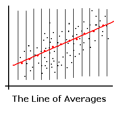
- The regression line can be thought of as a line of averages.
It connects the averages of the y-values in each thin vertical strip:

- The regression line is the line that minimizes the sum of the squares
of the residuals. For this reason, it is also called the
least squares line and the linear trend line.
- The R-squared value r2 has a special meaning. It is the proportion of variation in the dependent
variable that is explained by the independent variable.
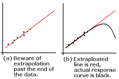
- Beware of extrapolating beyond the range of the data points.
The actual response curve may curve in an unexpected way.

Predicted Values and Residuals
- The actual value of the dependent variable is yi.
- The predicted value of yi is defined to be
y^i = a xi + b, where
y = a x + b is the regression equation.
- The residual is the error that is not explained by the
regression equation:
ei = yi -
y^i.
- A residual plot plots the residuals on the y-axis vs. the
predicted values of the dependent variable on the x-axis. We would like
the residuals to be
unbiased: have an average value of zero in any thin vertical
strip, and
homoscedastic, which means "same stretch": the spread of the
residuals should be the same in any thin vertical strip.
- The residuals are heteroscedastic if they are not
homoscedastic.
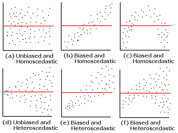
- Here are six residual plots and their interpretations:

- Unbiased and homoscedastic. The residuals average to zero in each
thin verical strip and the SD is the same all across the plot.
- Biased and homoscedastic. The residuals show a linear pattern,
probably due to a lurking variable not included in the experiment.
- Biased and homoscedastic. The residuals show a quadratic pattern,
possibly because of a nonlinear relationship. Sometimes a variable
transform will eliminate the bias.
- Unbiased, but homoscedastic. The SD is small to the
left of the plot and large to the right: the residuals are heteroscadastic.
- Biased and heteroscedastic. The pattern is linear.
- Biased and heteroscedastic. The pattern is quadratic.
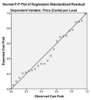
- We also like the residuals to be normally distributed. We
check this by looking at the normal plot of the residuals.
- Why is the R-squared value the proportion of variation due to the independent variable?
Ans: Because the variation due to the independent variable is
Sum of Squares due to Model = SSM = (y^1 -
y)2 + ... +
(y^n - y)2
On the other hand, the
Sum of Squares due to Error = SSE = (y1 - y^1)2 + ... +
(yn - y^n)2.
If we define Sum of Squares Total = SST = (y1 - y)2 + ... +
(yn - y)2),
it can be shown that SST = SSM + SSE, and that r2 = SSM / SST = SSM / (SSM + SSE),
which is the proportion of the variation due to the independent variable.
Regression with SPSS
- With the Laundry Dataset, use SPSS to display the scatterplot of price (y-axis) vs.
rating (x-axis):
- Import the Laundry Dataset dataset into SPSS.
- Verify that for the variables Rating and Price, Type is set to Numeric and Measure to Scale.
- Set the labels for Rating and Price to "Consumer Union Rating" and "Price (Cents) per Load", respectively.
- Find the simple regression equation for predicting Price from Rating:
- Select Analyze >> Regression >> Linear
Drag the Rating variable into the Independent(s) box.
Drag the Price variable into the Dependent box.
Click OK.
Click the Plots button.
Click OK.
- In the Coefficients box, the unstandardized B values are -2.144 for
(Constant) and 0.373 for
Consumer Union Rating. The regression equation is
therefore:
Price = 0.373 * Rating - 2.144
- There are two methods or creating the residual plot and the normal plot of the residuals.
(I prefer Method 2).
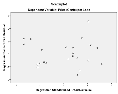
- Method 1, create the plots with the SPSS ZPRED and ZRESID variables:
Select Analyze >> Regression >> Linear
The Rating and Price variables should already be in the
Independent(s) and Dependent boxes.
Click the Plots button.
Move ZRESID into the Y box in Scatter 1 of 1.
Move ZPRED into the X box in Scatter 1 of 1.
Check Normal Probability Plot in
the Standardized Residual Plots box.
Click Continue; Click OK.
- Resulting residual plot:

- Resulting normal plot of residuals:
;

- Method 2, save the unstandardized residuals and predicted values:
Select Analyze >> Regression >> Linear
The Rating and Price variables should already be in the
Independent(s) and Dependent boxes.
Click the Save button.
In the Linear Regression: Save Dialog, check the boxes for Unstandardized
Predicted Value and Unstandardized Residuals.
Click Continue; Click OK.
The variables PRE_1 (Predicted Values) and RES_1 (Residuals) have been created in the dataset.
You can now create a scatterplot of the Unstandardized Residuals (y-axis) vs.
Unstandardized Predicted Values (x-axis) by using Graphs
>> ChartBuilder
Also create the normal plot of RES_1 (Residuals) with Analyze >> Descriptive
Statistics >> Q-Q Plots.
Root Mean Square Error
- The root mean square error (RMSE) for a regression model is
similar to the standard deviation (SD) for the ideal measurement model.
- We can write this as a Miller analogy:
RMSE : regression model :: SD : ideal measurement model
- The SD estimates the deviation from the sample mean
x.
- The RMSE estimates the deviation of the actual y-values from the
regression line. Another way to say this is that it estimates the standard deviation
of the y-values in a thin vertical rectangle.
- The RMSE is computed as
RMSE = √[(
e12 +
e22 + ... +
en2) / n]
where ei = yi -
yi^.
- The RMSE can be computed more simply as
RMSE = SDy
√(1 - r2).
- Example: If SDy = 30 and
r = 0.6, then
RMSE = SDy
√(1 - r2) = 30 *
√(1 - 0.42) = 30 * 0.6 = 18.
- You may wonder where the formula RMSE = SDy √(1 - r2) comes from. Here is a short explanation:
SSM + SSE = SST
SSE = SST - SSM
SSE / n = SST / n - (SST * SSM) / (SST / n)
MSE = Var(n) - Var(n) * (SSM / SST)
MSE = Var(n) - Var(n) * r2
MSE = Var(n) (1 - r2)
√MSE = √Var(n) √(1 - r2)
RMSE = SDy √(1 - r2)
MSE means mean squared error; RMSE is the square root of MSE = root mean
squared error.
