To Notes

IT 223 -- Jan 28, 2026

Review Exercises

  1. What is the standard normal density?
    Answer: It is a normal density with center μ = 1 and spread σ = 1.
  2. IQ scores are normally distributed with mean = 100 and SD=15. How many persons out of 100 have an IQ score greater than 120?
    Answer: First compute the z-score z = (120 - 100) / 15 = 20 / 15 = 1.33.
    Then area[1.33, ∞) = 1 - area(-∞, 1.33] = 1 - 0.9082 = 0.0918 = 9%. Here is the R calculation:
    (1 - pnorm(120, mean=100, sd=15) 
    [1] 0.09121122
    
  3. IQ scores are normally distributed with mean = 100 and SD = 15. How many persons out of one billion have an IQ score greater than 175? Use the Extreme Values of the Normal Distribution table.
    Answer: z = (x - mu) / sigma = (175 - 100) / 15 = 5. to see that the proportion of scores greater than 5 is 2.867 × 10⁻⁷. Multiply this proportion by 1 billion = 109 to see how many persons out of one billion have an IQ score greater than 175:
    2.867 × 10-7 * 109 = 286.7 ≈ 287. The R calculation:
    (1 - pnorm(175, mean=100, sd=15)) * 1.0e9
    [1] 286.6516
    
  4. What is the 90th percentile for IQ scores. mean = 100 and SD = 15 for IQ scores.
    Answer: look up 0.9 in the second normal table and read the z-value in the margins of the table 1.28. Then convert this z-value to an IQ score: z * sd + mean = 1.28 * 15 + 100 = 119.2. The R calculation:
     qnorm(0.9, mean=100, sd=15)
    [1] 119.2233
    
  5. What are the definitions of unbiased, biased, homoscedastic, and heteroscedastic. Answer: look at a plot of data points vs. observation number.
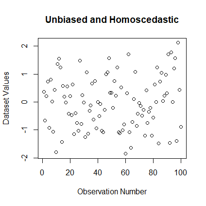
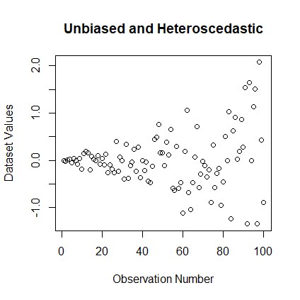
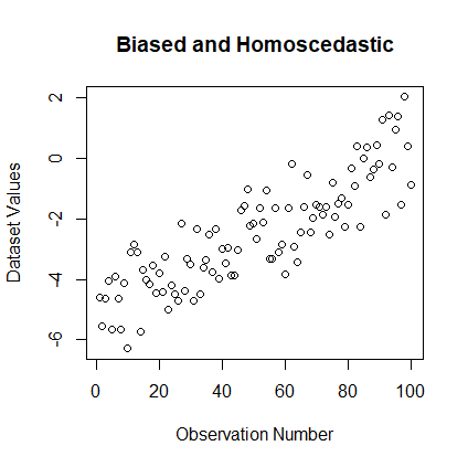
    Unbiased means the data have the same mean in any thin rectangle all the way across the plot.
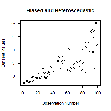
    Biased means the data do not have the same mean in every thin rectangle.
    Homoscedastic means that the data have the same standard deviation in every thin rectangle.
    Heteroscedastic means that the data do not have the same SD in every thin rectangle.
  6. four Set up the R vector x with values from 1 to 200 and the R vector y that contains 200 standard normal random values. Then create separate plots for y1, y2, y3, and y4 all vs. x for these R definitions:
    y1 <- y
    y2 <- y * (x / 100)
    y3 <- y + (x - 100) * 0.05
    y4 <- y * x / 100 + (x - 100) * 0.025
    
    Classify each plot as unbiased or biased; homoscedastic or heteroscedastic.
    Answer: set up the vector of observation numbers and normal random values:
    x <- 1:100
    y <- rnorm(100)
    
    Then create four plots:
    Plot 1:
    > y1 <- y
    > plot(x, y1, xlab="Observation Number",
    + ylab="Dataset Values", 
    + main="Unbiased and Homoscedastic")
    
    Plot1 : Unbiased and Homoscedastic

    Plot 2:
    > y2 <- y * (x / 100)
    > plot(x, y2, xlab="Observation Number",
    + ylab="Dataset Values",
    + main="Unbiased and Heteroscedastic")
    
    Plot2 : Unbiased and Heteroscedastic

    Plot 3:
    y3 <- y + (x - 100) * 0.025
    plot(x, y3, xlab="Observation Number", 
    + ylab="Dataset Values",
    + main="Biased and Homoscedastic")
    
    Plot 3 : Biased and Homoscedastic

    Plot 4:
    > y4 <- y * x / 100 + (x - 100) * 0.025
    > plot(x, y4, xlab="Observation Number", 
    + ylab="Dataset Values",
    + main="Biased and Heteroscedastic")
    
    Plot4 : Biased and Heteroscedastic

Normal Plots

Practice Problems

  1. Compute normal scores for a dataset of size 9.
    Answer: Choose the z-scores that divide the standard normal curve into 9 + 1 = 10 equal areas:
    -1.28  -0.84  -0.52  -0.25  0.00  0.25  0.52  0.84  1.28
  2. Construct the normal plots by hand of this dataset:
     
           81   95   97   101   112   125   129   167   220
  3. Create the normal plot for this dataset with R. Answer:
    > x <- c(81, 95, 97, 101, 112, 125, 129, 167, 220)
    > qqnorm(x)
    

    Normal Plot 1

R Practice Problems

  1. Create 50 values of a normal random variable x with μ = 15, σ = 3.8.
    1. Create a histogram of x.
    2. Create a normal plot of x.
    Answer:
    > x <- rnorm(50, mean=15, sd=3.8)
    > hist(x)
    > qqnorm(x)
    
  2. Create 50 values of a uniform random variable x in the range [10, 50]:
    > x <- runif(50, min=10, max=50)
    
    1. Create a histogram of x.
    2. Create a normal plot of x.
    Answer:
    > x <- runif(50, min=10, max=50)
    > hist(x)
    > qqnorm(x)
    

Bivariate Datasets