Linear Regression

The Regression Equation

Example: A dataset consists of heights (x-variable) and weights (y-variable) of 977 men, of ages 18-24. Here are the summary statistics:
      x = 70 inches    SD_x+ = 3 inches
      y = 162 pounds    SD_y+ = 30 pounds
      r_xy = 0.5
We want to derive an equation, called the regression equation for predicting y from x.
If x increases above x = 70 by one SD_x = 3, how much will y increase, on the average?
Answer: it depends on the correlation r. What happens with these three scenerios?
1. r = 0.0
2. r = 1.0
3. r = 0.5
In general, here is the formula for the regression equation:
y - y = (r SD_y / SD_x)(x - x)
Use this formula to derive the regression equation for the example at the top of this page. Answer:
      y - y = (r SD_y / SD_x)(x - x)
      y - 162 = (0.5 * 30 / 3)(x - 70)
      y - 162 = 5 * (x - 70)
      y = 5x + 350 - 162
      y = 5x - 188
5 is the slope = a^{^}, -188 is the intercept = b^{^}.
What are the predicted weights for these heights?
76 67 70
Answer:
y^{^} = a^{^} * x + b^{^} = 5 * 76 - 188 = 192
y^{^} = a^{^} * x + b^{^} = 5 * 67 - 188 = 147
y^{^} = a^{^} * x + b^{^} = 5 * 70 - 188 = 162
The regression line can be thought of as a line of averages. It connects the averages of the y-values in each thin vertical strip:
The regression line is the line that minimizes the sum of the squares of the residuals. For this reason, it is also called the least squares line and the linear trend line.
The R-squared value r² has a special meaning. It is the proportion of variation in the dependent variable that is explained by the independent variable.
Beware of extrapolating beyond the range of the data points. The actual response curve may curve in an unexpected way.

Predicted Values and Residuals

The actual value of the dependent variable is y_i.
The predicted value of y_i is defined to be y^{^}_i = a x_i + b, where y = a x + b is the regression equation.
The residual is the error that is not explained by the regression equation:
e_i = y_i - y^{^}_i.
A residual plot plots the residuals on the y-axis vs. the predicted values of the dependent variable on the x-axis. We would like the residuals to be
unbiased: have an average value of zero in any thin vertical strip, and
homoscedastic, which means "same stretch": the spread of the residuals should be the same in any thin vertical strip.
The residuals are heteroscedastic if they are not homoscedastic.
Here are six residual plots and their interpretations:
1. Unbiased and homoscedastic. The residuals average to zero in each thin verical strip and the SD is the same all across the plot.
2. Biased and homoscedastic. The residuals show a linear pattern, probably due to a lurking variable not included in the experiment.
3. Biased and homoscedastic. The residuals show a quadratic pattern, possibly because of a nonlinear relationship. Sometimes a variable transform will eliminate the bias.
4. Unbiased, but homoscedastic. The SD is small to the left of the plot and large to the right: the residuals are heteroscadastic.
5. Biased and heteroscedastic. The pattern is linear.
6. Biased and heteroscedastic. The pattern is quadratic.
We also like the residuals to be normally distributed. We check this by looking at the normal plot of the residuals.
Why is the R-squared value the proportion of variation due to the independent variable?
Ans: Because the variation due to the independent variable is
Sum of Squares due to Model = SSM = (y^{^}₁ - y)² + ... + (y^{^}_n - y)²
On the other hand, the
Sum of Squares due to Error = SSE = (y₁ - y^{^}₁)² + ... + (y_n - y^{^}_n)².
If we define Sum of Squares Total = SST = (y₁ - y)² + ... + (y_n - y)²,
it can be shown that SST = SSM + SSE, and that r² = SSM / SST = SSM / (SSM + SSE),
which is the proportion of the variation due to the independent variable.

Regression with R

For each question, show to the R source code and the R output and graphs.

Read the CSV file laundry-detergent.txt from the computer harddrive. Save it as an R dataset with variables Rating and Price: laundry-detergent.txt

> setwd("c:/it223")
> getwd( )
[1] "d:/it223"
> laundry_df <- read.csv("laundry-detergent.txt", header=T)
> print(laundary_df)
1 61 17
2 55 30
3 50 9
4 46 13
5 35 8
6 32 5
7 59 22
8 52 23
9 48 16
10 46 13
11 34 12
12 29 14
13 56 22
14 51 11
15 48 15
16 45 17
17 33 7
18 26 11
19 55 16
20 50 15
21 48 18
22 36 8
23 32 6
24 26 13

From the Laundry Data Frame, print the Rating and Price variables separately:

> print(laundry_df$Rating)
[1]  61 55 50 46 35 32 59 52 48 46 34 29
[13] 56 51 48 45 33 26 55 50 48 36 32 26
> print(laundry_df$Price)
[1]  17 30  9 13  8  5 22 23 16 13 12 14 
[13] 22 11 15 17  7 11 16 15 18  8  6 13

With the Laundry Detergent Dataset, use R to display the scatterplot of price (y-axis) vs. rating (x-axis).

Find the correlation of Rating with Price.

> cor(laundry_df$Rating, laundry_df$Price)
[1] 0.6707535

Find the simple regression equation for predicting Price from Rating.

> model <- lm(Price ~ Rating, data=laundry_df)
> model

Call:
lm(formula = Price ~ Rating, data = laundry_df)

Coefficients:
(Intercept) Rating 
-2.1443 0.3727

The regression equation is y = 0.3727x - 2.1443.

Print the summary statistics of the regression model.

> summary(model)

Call:
lm(formula = Price ~ Rating, data = laundry_df)

Residuals:
Min 1Q Median 3Q Max 
-7.491 -3.185 -1.119 2.597 11.645 

Coefficients:
Estimate Std. Error t value Pr(>|t|) 
(Intercept) -2.14435 3.96484 -0.541 0.594051 
Rating 0.37271 0.08786 4.242 0.000334 ***
---
Signif. codes: 0 ‘***’ 0.001 ‘**’ 0.01 ‘*’ 0.05 ‘.’ 0.1 ‘ ’ 1

Residual standard error: 4.539 on 22 degrees of freedom
Multiple R-squared: 0.4499, Adjusted R-squared: 0.4249 
F-statistic: 17.99 on 1 and 22 DF, p-value: 0.0003342

Obtain the residuals e_i = y_i - y^{^}_i, i=1,...,n for the simple regression model.

> res <- predict(model)
> res
         1          2          3          4 
-3.5910035 11.6452605 -7.4911862 -2.0003435 
         5          6          7          8 
-2.9005262 -4.7823942  2.1544178  5.7633925 
         9         10         11         12 
 0.2542352 -2.0003435  1.4721845  5.3357378 
        13         14         15         16 
 3.2725498 -5.8638968 -0.7457648  2.3723672 
        17         18         19         20 
-3.1551048  3.4538698 -2.3547395 -1.4911862 
        21         22         23         24 
 2.2542352 -3.2732368 -3.7823942  5.4538698

Obtain the predicted values y^{^}_i from the linear regression model.

> pred <- predict(model)
> pred
        1         2         3         4 
20.591003 18.354739 16.491186 15.000343 
        5         6         7         8 
10.900526  9.782394 19.845582 17.236607 
        9        10        11        12 
15.745765 15.000343 10.527816  8.664262 
       13        14        15        16 
18.727450 16.863897 15.745765 14.627633 
       17        18        19        20 
10.155105  7.546130 18.354739 16.491186 
       21        22        23        24 
15.745765 11.273237  9.782394  7.546130

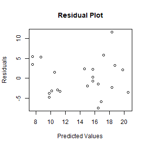
Plot the residuals vs. predicted values for your regression model.

> plot(pred, res, xlab="Predicted Values", ylab="Residuals",
+     main="Normal Plot of Residuals")

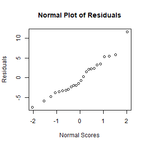
Obtain a normal plot of the residuals.

> plot(resid, main="Normal Plot of Residuals")

Root Mean Square Error

The root mean square error (RMSE) for a regression model is similar to the standard deviation (SD) for the ideal measurement model.
We can write this as a Miller analogy:
RMSE : regression model :: SD : ideal measurement model
The SD estimates the deviation from the sample mean x.
The RMSE estimates the deviation of the actual y-values from the regression line. Another way to say this is that it estimates the standard deviation of the y-values in a thin vertical rectangle.
The RMSE is computed as
RMSE = √[( e₁² + e₂² + ... + e_n²) / n]
where e_i = y_i - y_i^{^}.
The RMSE can be computed more simply as RMSE = SD_y √(1 - r²).
Example: If SD_y = 30 and r = 0.6, then
RMSE = SD_y √(1 - r²) = 30 * √(1 - 0.4²) = 30 * 0.6 = 18.
You may wonder where the formula RMSE = SD_y √(1 - r²) comes from. Here is a short explanation:
      SSM + SSE = SST
      SSE = SST - SSM
      SSE / n = SST / n - (SST * SSM) / (SST / n)
      MSE = Var(n) - Var(n) * (SSM / SST)
      MSE = Var(n) - Var(n) * r²
      MSE = Var(n) (1 - r²)
      √MSE = √Var(n) √(1 - r²)
      RMSE = SD_y √(1 - r²)
MSE means mean squared error; RMSE is the square root of MSE = root mean squared error.