To Lecture Notes

CSC 433 -- May 15, 2017

Quiz 7

• Take Quiz 7 in groups of 2 or 3.

Review Exercises

1. What does numeric(0) mean? What do you think numeric(n) means?
    
2. How do you create a vector having length 0 of the following types: character, numeric, logical?
   Ans: v1 = character(0)  v2 = numeric(0)  v3 = logical(0).
    
3. For the list xx defined by
   

   xx <- list(name="Alice", gender="F", age=11)
   

   How do you access the items in a list by index?
   Ans: xx[[1]], xx[[2]], xx[[3]]
   Here is an interactive session:
   

   > xx <- list(name="Alice", gender="M", age=11)
   > xx
   $name
   [1] "Alice"
   
   $gender
   [1] "M"
   
   $age
   [1] 11
   
   > print(xx[[1]])
   [1] "Alice"
   
   > print(xx$name)
   [1] "Alice"
   

4. Create a list of 26 dataframes with one row each:
   

      num letter  
   1   1      A
   
     num letter
   1   2      B
   
   ...
   
     num letter
   1  26      Z  
   

   Ans: Here is the script (improved from the one given in class):
   

   biglist <- NULL
   for(i in 1:26) {
      biglist[[i]] <- data.frame(num=i, 
         letter=rawToChar(as.raw(64+i)))
   }
   print(biglist)
   

5. Redo the MyConcat example so that the myConcat function looks similar to the myCbind function for Project 5. Also write a function named runTimings that returns a dataframe containing the times for the slow function myConcat and the fast function c. Ans:
   

   myConcat <- function(u, v) {
      lenu <- length(u)
      lenv <- length(v)
      w = rep(0, lenu + lenv)
      for(i in 1:lenu) {
         w[i] = u[i]
      }
      for(i in 1:lenv) {
         w[i + lenu] = v[i]
      }
      return(w)
   }
   
   runTimings <- function( ) {
      df <- data.frame(size=numeric(0), 
         fast=numeric(0), slow=numeric(0))
      for(n in seq(50000, 250000, 50000)) {
         u = runif(n)
         v = runif(n)
         times <- system.time(c(u, v))
         fast_time = as.vector(times[3])
         times <- system.time(myConcat(u, v))
         slow_time = as.vector(times[3])
         df <- rbind(df, data.frame(size=n, 
            fast=fast_time, slow=slow_time))
      }
      return(df)
   }
   

6. Sort the rows of the dataframe from the Kids1 Example by (a) name, (b) age, (c) descending age, (d) gender, descending age, and name. Use the order function, not the sort function. Ans:
   

   kids <- read.table("c:/datasets/kids1.txt", header=T)
   kids[order(kids$name), ]
   kids[order(kids$age), ]
   kids[order(-kids$age), ]
   kids[order(kids$gender, -kids$age, kids$name), ]

7. Set up a plotting area like this. Then add these items to the plot:
    
   
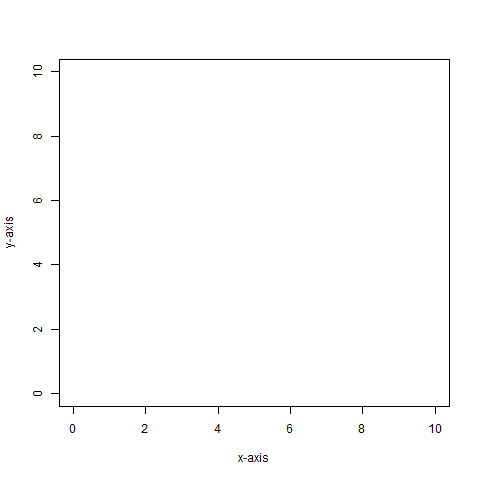
   1. The points (2, 3), (5, 1), (8, 8) plotted with red plotting symbols pch=16.
       
   2. The polyline defined by (1, 9), (1, 1), (8, 8).
       
   3. The string "Start Point" centered at (2, 1).
   
   Ans:
   

   plot(NULL, NULL, xlim=c(0, 10), ylim=c(0, 10),
      xlab="x-axis", ylab="y-axis")
   points(c(2, 5, 8), c(3, 1, 8), pch=16, col="red")
   lines(c(1, 1, 8), c(9, 1, 8))
   text(2, 1, "Start Point")
   

   
   
8. Try out the str and summary functions on a data frame created from kids1.txt.
   Ans: The str function shows the structure of an object:
   

   > str(kids)
   'data.frame': 2 obs. of 3 variables:
   $ name  : Factor w/ 2 levels "Alice","Bob": 1 2
   $ gender: Factor w/ 2 levels "F","M": 1 2
   $ age   : int  11 12
   

   The summary function is similar. It summarizes the data in an object:
   

   > summary(kids)
   name     gender   age 
   Alice:1  F:1      Min. :11.00 
   Bob  :1  M:1 1st  Qu.:11.25 
                     Median :11.50 
                     Mean :11.50 
                     3rd Qu.:11.75 
                     Max. :12.00
   

9. An anonymous function is an R function that is not assigned a name like this:
   

   (function(x)sum(x^2))(1:10)
   

   (The normal way to use such a function is like this:
   

   sumOfSquares <- function(x) {
      sum(x^2)
   }
   print(sumOfSquares(1:10))
   

   Give an example of where anonymous functions are useful in R.
   Ans: The apply function where you apply a function to rows of a matrix or dataframe.
    
10. What does brushing mean when referring to statistical graphics? Look again at the BodyBrain Example.
    Ans: It means clicking on or mousing over points in a scatterplot to get more information about those points, such as observation numbers, labels, or corresponding points in other plots.
     
11. True/False: you can create an R factor from numeric data.
    Ans: True. A factor represents categorical data. You can use numbers to represent categorical data.
     
12. We will discuss this problem next week on May 22.
    
    Use R to compute the 0.63 quartile = Q(0.63) for the vector
    

    v <- c(45, 31, 19, 76, 111)
    

    using methods 1 and 4. Verify your results by hand.
    Ans: First sort the vector:
    

    19  21  45  76   111
    

    Compute the 0.67 quartile = Q(0.67) using Method 1:
    We have
     
    

    Index:	1	2	3	4	5
    Quantile:	0.2	0.4	0.6	0.8	1.0
    Value:	x1=19	x2=21	x3=45	x4=76	x5=111

    
    To find the 0.67 quartile, note that 0.67 is between quantile 0.6 and 0.8 in the table--we round up to 0.8, so Q(0.67) = x₄ = 76.
     
    Compute Q(0.67) using Method 4:
    Using the table above we see that Q(0.6) = x₃ = 45 and Q(0.8) = x₄ = 76. Use linear interpolation to find Q(0.67)
     
    
     
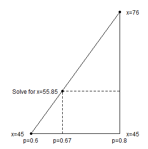
    We use similar triangles:
     
    
    (x - 45) / (76 - 45) = (0.67 - 0.6) / (0.8 - 0.6)
     
    (x - 45) / 31 = 0.07 / 0.2
     
    x = 31 * 0.07 / 0.2 + 45 = 55.85
    
    Check with R:
    

    > quantile(v, 0.67, type=1)
    67% 
    76 
    > quantile(v, 0.67, type=4)
    67% 
    55.85 
    > 
    

    Here is the R script that draws the interpolation diagram.
     
    See the Quantile Computations document for the details of computing quantiles of types 1 to 9.

• Know these R graphics parameters for the final exam:
   
  

   cex  cex.axis  cex.lab  cex.main  
  
  cex.sub  col  lty  main  pch  sub  
  
  type  xlim  xlog  ylim  ylog
  

Defining Your Own R Classes

• R maintains two types of classes: S3 and S4 classes.
   
• The preferred class definition for new code is S4.
   
• The older S3 classes are maintained for backward compatability with S code.
   
• Most of the R packages available for download on CRAN use S3 classes.
   
• Details about S3 and S4 classes (We only discuss S3 classes in this class.)
   
• The Die and Infant examples show how to implement S3 classes.
   
• Here are some commonly used S3 classes:
  

  data.frame  Date  ts
  

• matrix is a special non-S3 class.
   
• For Project 7, you will implement an S3 class.

R Date Objects

• R Date object will be discussed next week on May 23.
   
• The R Date class represents a date or a date and time.
   
• Some R DateTime Classes

R Timeseries Objects

• R timeseries objects will be discussed next week on May 23.
   
• The ts class represents timeseries objects. It comes with the basic R installation.
   
• The ts Class
   
• The zoo and xts packages can handle not only dates but also datetime values.

Functions Associated with Probability Distributions and Densities

• A random variable is a process for generating random outcomes.
   
• A discrete random variable has a finite or countably infinite set of possible outcomes.
   
• A continuous random variable has outcomes in an interval, finite or infinite.
   
• We only consider the three families of continuous random variables, normal, uniform, and exponential:
   
  
  A normal random variable X has outcomes in the interval (-∞, +∞).
   
  A uniform random variable U has outcomes in the interval [a, b]; a is the minimum value of U; b is the maximum value of U.
   
  An exponential random variable T has outcomes in the interval [0, +∞).
  
  
• SAS and R have functions for describing other a wide variery of discrete and continuous variables, including Bernoulli, Beta, Cauchy, Chi-Square, F, Gamma, Generalized Poisson, Geometric, Hypergeometric, Laplace, Logistic, Lognormal, Negative Binomial, Normal Mixture, Pareto, Poisson, T, Tweedie, Wald (Inverse Gaussian), Weibull.
   
• R functions related to the Normal, Uniform, and Exponential distributions:
   
  

  Density	Prob(X ≤ s)	Height of Density	Quantile: q such that Prob(X ≤ q) = p	Outcome of Random Variable
  Normal	pnorm(s, m, sd)	dnorm(x, m, sd)	qnorm(p, m, sd)	rnorm(n, m, sd)
  Uniform	punif(s, a, b)	dunif(u, a, b)	qunif(p, a, b)	runif(n, a, b)
  Exponential	pexp(s, r)	dexp(t, r)	qexp(p, r)	rexp(n, r)

  
   
• For information about SAS functions for Cumulative Probabability Distribution Functions, Probability Densities, Quantiles, and Random Number Generators, see the corresponding link.
   
• Practice Problems
   
  
  1. Use the pnorm function to compute the probability of being within 1, 2, or 3 standard deviations of the mean. Ans:
     

      > print(pnorm(1:3, mean=0, sd=1) - 
             pnorm(-(1:3), mean=0, sd=1))
     [1] 0.6826895 0.9544997 0.9973002
     

  2. Use the qnorm function to find a 95% confidence interval for the normal distribution. Ans:
     

     > print(qnorm(0.975, mean=0, sd=1)
     [1] 1.959964
     

  3. What is the standard deviation of Uniform[3, 5] random variables? Ans: Generate 100,000 random outcomes from this distribution:
     

     > u <- runif(100000, 3, 5)
     > print(sd(u))
     [1] 0.5777419 
     

     If U is a uniform(3, 5) random variable, the theoretical variance is
      
     
     E((U - E(U))²) = E((U - 0.5)²) = ∫₃⁵(u - 0.5)²(1/2)du = ∫_-1¹ w²(1/2)dw = 1/3
     
     The theoretical standard deviation is √1/3 = 0.5773503.

A Simulated Bivariate Normal Dataset

• The normal distribution is popular because it occurs often in nature and in financial applications. The dataset from the SAS Pearson Example is an example of a bivariate dataset. Use R to create a scatterplot of the son's height vs. the father's height.
   
• R is convenient for simulations using hypothetical random data.
   
• Example: Create a dataframe with n simulated random normal observations according to these specifications:
   
  
  μ_x = 2   σ_x² = 9     μ_y = 1   σ_y² = 4     σ_xy = 3.6 
  
  
  For the following discussion, use these definitions:
   
  
  E(x) = μ_x   Var(x) = σ_x²   E(y) = μ_y   Var(y) = σ_y²   Cov(x, y) = σ_xy
  
  Use these facts to help you write your script:
   
  
  E(x + y) = E(x) + E(y)     E(aX) = aE(x)     Var(ax) = a²Var(bx)
   
  Var(x + y) = Var(x) + 2Cov(x, y) + Var(y)
  
  When you have finished generating the data frame, plot it.
   
  The correlation of the two datasets is
   
  
  ρ_xy = σ_xy / (σ_x σ_y) = 3.6 / (3 * 2) = 0.6.
  
  First create two sets of 40 independent standard normally distributed random observations:
  

  u = rnorm(40, mean=0, sd=1)
  v = rnorm(40, mean=0, sd=1)
  

  Now create w as a linear combination of u and v:
  

  w = 0.6 * u + sqrt(1 - 0.6^2) * v
  

  Recall that
   
  
  Cov(x, ay + bz) = a Cov(x, y) + b Cov(x, z)
   
  Cov(x, x) = Var(x) Var(x + y) = Var(x) + 2 Cov(x, y) + Var(y)
   
  Var(ax) = a² Var(x)
  
  The factors 0.6 and sqrt(1 - 0.6) are chosen so that w will have the correct correlation of 0.6 with u and the correct variance of 1:
   
  
  Cov(u, v) = Cov(u, ru + √(1 - r²)v) = r Cov(u, v) + √(1 - r²) Cov(u, v)
   
           = r × Var(u) + √(1 - r²) × Cov(u, v) = r,
  
  because Var(u) = 1 and Cov(u, v) = 0 (u and v are independent). Also
   
  
  Var(w) = Var(ru + √(1 - r²) v) = Var(ru) + 2 Cov(ru, √(1 - r²) v) + Var(√(1 - r²) v)
   
           = r² Var(u) + 2 r√(1 - r²) Cov(u, v) + √(1 - r²)² Var(v)
   
           = r² 1 + 2 r√(1 - r²) 0 + √(1 - r²)² 1 = r² + 1 - r² = 1
  
  Then transform u and w so that they have the correct variances and covariance. Here is the entire script for creating and plotting the simulated bivariate normal vector:
  

  # Create two standard normal 
  # independent vectors.
  u = rnorm(40, mean=0, sd=1)
  v = rnorm(40, mean=0, sd=1)
  
  # Create a vector w that has a 
  # correlation of 0.6 with u, such
  # that w is still standard normal.
  w = 0.6 * u + sqrt(1 - 0.6^2) * v
  
  # Set means and standard 
  # deviations to specified values.
  mux = 2
  sigmax = 3
  muy = 1
  sigmay = 2
  
  # Scale x and y so that they
  # have the correct means and SDs.
  x = sigmax * u + mux
  y = sigmay * w + muy
  
  # Plot the resulting points defined
  # by the vectors x and y.
  plot(x, y)