To Lecture Notes

CSC 423 -- 7/19/17

Review Exercises

1. What is the standard normal density?
   Ans: A normal density with population mean μ=0 and variance σ=1. (Recall that the population (or sample) variance is the population (or sample) standard deviation squared. The standard normal distribution is denoted by N(0, 1). We abbreviate the statement that z is a N(0, 1) random variable as z ∼ N(0, 1).
    
2. What do inflection points have to do with the standard deviation of a normal density?
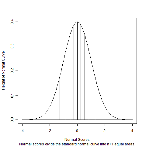
   Ans: A critical point is a point x on a curve where the first derivative f'(x) = 0, that is where the tangent line to the curve is horizontal, and x is a relative minimum or maximum. For a standard normal density, x = 0, the center of the density. This center is also the mean and the median. An inflection point is a point on the curve where the second derivative f"(x) = 0, where the curve changes from concave up to concave down, or vice versa. A normal density has inflection points at x = μ - σ and μ + σ. Thus the population standard deviation σ can be defined as the distance from the critical point to either of the inflection points.
    
3. What is a z-score?
   Ans: If the mean μ and standard deviation σ are known for a dataset, compute the z-score of a data point x like this: z = (x - μ) / σ. For example, IQ scores are scaled so that μ = 100 and σ = 15, so the z-score for an IQ score x is computed as
    
   
   z = (x - 100) / 15
   
   If μ and σ are not known, use the sample mean and standard deviation instead to compute the z-score: z = (x - x)/s_x. To compute the z-score for one of the sample means in a sequence of repeated experiments, use
    
   
   z = (x - μ) / SE_mean
   
   where SE_mean = s_x / √n
    
4. If z ∼ N(0, 1), use SAS and R to verify the probability that z is in each of these intervals:
    
   
   [-1, 1]    [-2, 2]    [-3, 3]
   
   Ans: Use the standard normal tables, which are the two tables in Table A: Standard Normal Probabilities. The first table is for negative z values; the second table is for positive z values. Compute the probability that z is in [-∞, 1] minus the probability that z in in [-∞, -1], which is 0.8413 - 0.1586 = 0.6827. Use similar calculations for [-2, 2] and [-3, 3]. This R session also computes the probabilities:
   

   > pnorm(1) - pnorm(-1)
   [1] 0.6826895  #<-- Matches the well 
                       known value 68%.
   > pnorm(2) - pnorm(-2)
   [1] 0.9544997  #<-- Matches the well 
                       known value 95%.
   > pnorm(3) - pnorm(-3)
   [1] 0.9973002  #<-- Matches the well 
                       known value 99.7%.
   > pnorm(4) - pnorm(-4)
   [1] 0.9999367  #<-- Very close to 1.
   

   You can also compute these four probabilities in one line as
   

   > pnorm(c(1, 2, 3) - pnorm(c(-1, -2, -3))
   [1] 0.6826895 0.9544997 0.9973002
   

   Here is how to compute these probabilites using a SAS script:
   

   * The cdf function means cumulative 
     distribution function;
   data probs;
      p1 = cdf("normal", 1) - cdf("normal", -1);
      output;
      p2 = cdf("normal", 2) - cdf("normal", -2);
      output;
      p3 = cdf("normal", 3) - cdf("normal", -3);
      output;
      
   proc print;
   run;
   

   Here is the SAS output:
   

       Obs       p
       1     0.68269
       2     0.95450
       3     0.99730
   

5. Use SAS and R to find a 99% confidence interval for z if z ∼ N(0,1).
   Ans: If the probability of a standard normal random variable being in [-z, z] is 0.95, then the probability of being in [-∞, z] is 0.975, because
    
   
   P(z in [-∞, -z]) = P(z in [-∞, -z]) = 0.025),
   so
    
   
   P(z in [-∞, z]) = P(z in [-∞, -z]) + P(z in [z, -z]) = 0.025 + 0.095 = 0.975.
   
   Looking up 0.975 in the body of the standard normal table, we find that the z corresponding to it is z = 1.96, so the 95% confidence interval is [-1.96, 1.96]. This can be computed with R like this:
   

   > qnorm(0.975)
   [1] 1.959964
   

   Similarly we find that a 99% confidence interval for z ∼ N(0, 1) is [-2.58, 2.58].
   Use this R script to find the 95 and 99% confidence intervals for z ∼ N(0, 1):
   

   qnorm(c(0.975, 0.995))
   
   Output:
   [1] 1.959964 2.575829
   

   Here is the corresponding SAS script and output:
   

    data confint;
      val = quantile("normal", 0.975);
      output;
      val = quantile("normal", 0.995);
      output;
   
   proc print;
   run;
   
   Output:
   Obs   val
    1  1.95996
    2  2.57583
   

6. What is the standard error of the sample mean? How do you compute it?
   Ans: The square root of the variance of the mean. It measures how variable the sample mean would be if you repeated the experiment many times. Compute the standard error of the mean with SE_mean = s_x / √x. See Property 9 in Section 6 of the Properties of Random Variables document for a derivation of the expression for SE_mean.
    
7. What is an outlier?
   Ans: An outlier is a point that is further than expected from the center of the distribution. The engineer's rule says that an outlier is a point with a z-score greater than 2 or less than -2. An extreme outlier is a point with a z-score greater than 3 or less than -3. A mild outlier is an outlier but is not an extreme outlier. Outliers can also be determined by looking at the boxplot, which was first proposed by John Tukey (1915 to 2000). In this case, an outlier is a point that is outside of the inner fences. where the inner fences are the points 1.5 IQRs below the 25%ile and 1.5 IQRs above the 75%ile.
    
8. (Not discussed in class, but you should know how a boxplot is constructed.) Draw the boxplot of these hypothetical exam scores:
    
   
   5  39  75  79  85  90  91  93  93  98
   
   See the NIST Example to see how to create boxplots with SAS or R.
   Ans: To draw the boxplot, we obtain the following information using the Tukey's Hinges method:
   Median = 50%ile = (85 + 90) / 2 = 87.5.
   Quartile 1 (Q1) = 25th%ile = Median of bottom half of sorted list = 75.
   Quartile 3 (Q3) = 75th%ile = Median of top half of sorted list = 93.
   If the sample size is odd, the middle value is used in both the top and bottom halves of the list.
   Inner quartile range = IQR = Q3 - Q1 = 93 - 75 = 18.
   Now construct the box plot; the bottom, middle, and top horizontal lines are Q1, Q2, and Q3, respectively.
    
   
    
   Now determine the inner and outer fences for the purpose of determining the outliers:
   The inner fences are located at
   Q1 - 1.5 * IQR = 75 - 1.5 * 18 = 48
   and Q3 + 1.5 * IQR = 93 - 1.5 * 18 = 120
   Any points that are outside of the inner fences are considered to be outliers.
   These points are 5 and 39. (There are no outliers above 120.)
    
   The outer fences are located at
   Q1 - 3 * IQR = 75 - 3 * 18 = 21
   and
   Q3 + 3 * IQR = 93 + 3 * 18 = 147
   Any points outside of the outer fence are considered to be extreme outliers and are marked with *.
   5 is the only extreme outlier.
    
   39 is an outlier, which is not an extreme outlier; it is considered to be a mild outlier and is marked with O.
   Normally vertical lines (whiskers) are drawn between Q3 and the lower inner fence, and between Q3 and the upper inner fence, but only if there are data points there.  There are no data points between the lower inner fence at 48 and the outlier at 39, so there is no whisker drawn between between 39 and 48.
    
   SAS code for drawing the boxplot:
   

   proc boxplot;
      plot scores * dummy /  boxstyle = schematic;
   

   The variable dummy is defined in the data step as 1 or some other arbitrary constant.
    
   R function call for drawing the boxplot:
   

   boxplot(scores)

   Here are the resulting SAS boxplot and R boxplot. Note that neither SAS nor R distinguishes between mild and extreme outliers. For both boxplots, all outliers are shown with an O symbol.
    
9. What are some important windows in the SAS for Windows version 9.4? How do you run a SAS script?
   Ans: Enhanced Editor, Log Window, Results Window (HTML and graphics output), Output Window (typewriter output).
    
10. Draw the histogram of the exam scores in Problem 8 with bin boundaries at 0, 20, 40, 60, 80, 100. Check your answer with SAS and R.
    Ans: (Not discussed in class, but you should know how a histogram is constructed.) Here is the histogram:
     
    
     
    SAS code for drawing the histogram:
    

    proc univariate noprint;
       histogram scores / endpoints = 
          (0, 20, 40, 60, 80, 100);
       
    or
    
    proc univariate noprint;
       histogram scores / endpoints = 
          (0 to 100 by 20);
    

    R function call for drawing the histogram:
    

    hist(scores, breaks=seq(0, 100, 20))
    

    Here are the resulting SAS histogram and R histogram.
     
11. Find the mistakes in these SAS statements:
    

    * Create dataset.
    data kids;
       infile kids.txt;
       input name, gender, age, firstobs=2;
    
    proc print data=kids
       
    proc means mean;
    

    The input file is c:\datasets\kids.txt, which contains
    

    Name Gender Age
    Sally  F    12
    Alex   M    11
    Jason  M     9
    Molly  F    10
    

    Ans: Here is the corrected version:
    

    * Create dataset;
    data kids;
       infile "c:/datasets/kids.txt" firstobs=2;
       input name $ gender $ age;
    
    proc print data=kids;  
    proc means mean;
    run;
    

12. How do you run an R script in RGui?
    Ans: Select the statements to run in the R script and enter Control-R, or right-click in the script window and select Run line or selection.
     
13. Write R statements to read the kids.txt file from the Question 12 into a data frame, print the data frame, and find the mean of the ages. Ans:
    

    kids = read.table("c:/datasets/kids.txt", header=TRUE)
    cat("kids data frame:\n")
    kids
    cat("Average age of kids:\n")
    mean(kids$Age)
    

    The R cat function literally outputs text to the console window. New line characters can be included as \n.

Final Project

• Look at the Final Project Description.

Normal Plots

• We know that a a normal distribution has an approximately bell-shaped histogram.
   
• in practice, it is often difficult to look at a histogram and determine how close its distribution is to normal, especially if the sample size n is small.
   
• An easier way to tell if a dataset is normally distributed is to look at the normal plot. If the normal plot is close to a straight line, the distribution of the dataset is close to normal.
   
• A normal plot is a scatterplot of the sorted actual data values (y-axis) vs. the expected normal scores (x-values).
   
• The NIST Example shows examples of normal plots in SAS and R.
   
• Here are sketches of five normal plots and their interpretations.
   
• If n is the number of observations, to compute the normal scores using Van der Waerden's method, find the z-scores that divide the standard normal curve into n + 1 equal areas.
   
• Practice Problem: Compute the normal scores of a dataset with 9 observations.
   
  Ans: The normal scores when n = 9 divide the standard normal curve into n + 1 = 10 equal areas like this:
   
  
   
  Look in the body of the normal table for these cumulative probabilities: 0.1000, 0.2000, 0.3000, 0.4000, 0.5000, 0.6000, 0.7000, 0.8000, and 0.9000. The closest matches are 0.5000, 0.5987, 0.6985, 0.7995, 0.8997. They have corresponding z-scores -1.28, -0.84, -0.52, -0.25, 0.00, 0.25, 0.52, 0.84, and 1.28. Here are three SAS and R scripts to find normal scores.  They both find the normal scores -1.2815516, -0.8416212, -0.5244005, -0.2533471, 0.0000000, 0.2533471, 0.5244005, 0.8416212, 1.2815516.
   
• Use the R function qqnorm to create a normal plot:
  

  > x = rnorm(200)
  > qqnorm(x)
  

• There exist formal tests of hypothesis to check if a given sample comes from a normal distribution. Sas provides the results of these tests with proc univariate.
   
• The NIST Example shows the SAS output of the Kolmogorov-Smirnov, Cramer-von Mises, and Anderson-Darling tests for normality.
   
• To interpret these tests at the 0.05 level of significance. If p < 0.05, reject the null hypothesis that the sample comes from a normal distribution; if p > 0.05, accept it.
   
• The problem with tests of normality in general is that it is difficult to find a test statistic that distinguishes normal from non-normal distributions in all cases, especially for small samples.
   
• Most statisticians find the normal plot to be more useful than tests of normality for checking whether a sample has an approximately normal distribution.

Tests of Hypothesis

• Some sample research questions:
   
  
  1. Do vaccines for children cause autism?
      
  2. Do the electric and magnetic fields in high voltage electric power lines cause health risks for those living nearby?
      
  3. Is there a difference in network traffic speed between our existing router, and the new router that management is considering?
      
  4. Is the level of mercury intake for wading birds in the Florida Everglades declining? (Mendenhall and Sincich, p. 49)
      
  5. Does being on a low-fat diet cause people to lose more weight than those on a regular diet? (Mendenhall and Sincich, p. 53)
      
  6. Do red light cameras installed in a traffic intersection affect the number of vehicle collisions in that intersection? (Mendenhall and Sincich, p. 53)
  
  
• These research questions phrased as null hypotheses:
   
  
  1. There is no significant difference between the rate of autism for vaccinated children vs. the rate of autism for non-vaccinated children?
      
  2. There is no significant difference between the incidence of cancer higher for persons living close to electric power lines vs. the rate of cancer for persons that to not live close to electric power lines?
      
  3. There is no significant difference in network traffic speed between our existing router and the proposed new router?
      
  4. There is no significant difference of mercury intake for wading birds in the Florida Everglades between last year and this year?
      
  5. There is no significance of difference in weight loss between people on a low-fat diet vs. those on a regular diet?
      
  6. There is no significant difference in the occurrence of vehicle crashes between those intersections that have red light cameras installed vs. those that do not.
  
  
• Usually the researcher wants to reject the null hypothesis to show that the effect being investigated causes a real difference, and is not just chance variation.

Some Terminology

• A simple random sample consists of randomly selected subjects from a population where every subject is equally likely to be selected.
   
• A treatment group is a group of subjects that are manipulated using a medicine, chemical, or other process being investigated.
   
• A control group is a special type of treatment group. It receives no special medicine, chemical, or process, but leaves the random sample as is.
   
• To prevent a patient from knowing whether he or she is in the treatment or control group, patients in clinical trials are usually given a placebo.
   
• A statistical experiment with two treatment groups can have a treatment group and a control group or two different treatment groups.
   
• The response variable is the outcome or measurement obtained from a statistical experiment.
   
• A one-sample test of hypothesis tests whether there is a significant difference between the responses of the treatment group and the responses of the general population.  The response of the population value is obtained from a previous studies, expert knowledge, or theoretical calculations.
   
• For a one-sample z- or t-test, the null hypothesis (H₀) states that the variation in the test statistic is just chance variation.
   
• For a one-sample z- or t-test, the alternative hypothesis (H₁) states that the the difference between the test statistic and zero is too large to plausibly be chance variation (the difference is significant).
   
• A two-sample test of hypothesis tests whether there is a significance between the responses of the two treatment groups.
   
  
  A paired two-sample test has a natural pairing between the subjects in the two treatment groups. Necessarily, in this case, the two groups must be the same size.
   
  An independent two sample test  has no natural pairing between the subjects. The two treatmant groups need not be the same size.
  
  
• For a two-sample test, the null hypothesis (H₀) states that the difference between the treatment groups is due to chance variation; there is no significant difference between the groups.
   
• For a two-sample test, the alternative hypothesis (H₁) states that difference between the treatment groups is too large to plausibly be chance variation (the difference is significant).
   
• A test statistic T is a value computed from the data and the null hypothesis. For a one-sample z-test, the test statistic is
   
  
  z = (x - μ) / SE_mean
  
  
• The level α of a test of hypothesis is the probability of rejecting H₀ if, in fact, H₀ is true. Traditionally, the level of a statistical test is taken to be 0.05 or 0.01.
   
• A 100(1-α)% confidence interval I is an interval such that T ∈ I 100(1-α)% of the time if H₀ is true.
   
• The p-value of a statistical test is the probability of obtaining a test statistic value as extreme or more extreme than the value actually obtained, given that H₀ is true.
   
• The rejection region for a statistical test is the set of values of the test statistic T that lead the researcher to reject the null hypothesis H₀ and accept the alternative hypothesis H₁. For any value of T in the rejection region, p < α, where p is the p-value and α is the level of the test.
   
• The acceptance region for a statistical test is the set of values of the test statistic T that lead the researcher to accept the null hypothesis H₀ and reject the alternative hypothesis H₁. For any value of T in the rejection region, p ≥ α, where p is the p-value and α is the level of the test. If H₀ is accepted, it does not necessarily mean that the researcher believes it is true, it may only mean that there is not enough evidence to reject H₀.
   
• The power of a statistical test is the probability of rejecting H₀ (whether is it is true or false). Increasing the sample size always increases the power of the standard statistical tests.

The Five Steps of a Hypothesis Test

1. State the null hypotheses H₀ and the alternative hypothesis H₁.
    
2. Compute the test statistic T.
    
3. Compute a (1-α)100% confidence interval I for the test statistic T, where α is the level of the hypothesis test.
    
4. If T ∈ I, accept H₀ (and reject H₁); if T ∉ I, reject H₁ (and accept H₀).
    
5. Compute the p-value for T. In most cases p must be computed using statistical software.

TTests of Hypothesis for One or Two Groups

• Descriptions of some tests of hypothesis for experimental designs that have one or two groups.
   
• Which t-test would you use, paired-sample t-test or independent two-sample t-test?
   
• Descriptions of tests with examples:
   
  
  1. One-sample z-test
      
  2. One-sample t-test
      
  3. Paired-sample t-test
      
  4. Independent Two-sample t-test
  
  
• There are two approaches to the independent two-sample t-test:
   
  
  1. Assume the variances of the two groups are equal, as described by the documents in the preceding link.
      
  2. Assume the variances can be different. This is called the Behrens-Fisher Problem, which we do not discuss in detail. Both SAS and R handle also handle the case of unequal variances. Both use Satterthwaite-Welch approximation, which can result in fractional degrees of freedom.

Overview of Regression

• Regression models will be discussed next week.
   
• A regression model is an equation that predicts the value of a dependent variable from zero or more independent variables
   
• Here are some examples of regression models that have been investigated in various disciplines (Mendenhall and Sincich, pp. 85 and 86):
   

Discipline	Dependent Variable	Independent Variables
History of Science	Height of adult child	Height of father, height of mother
Psychology	Aggressiveness of moonlighting employees	Age, gender, self-esteem, history of aggression supervisor abuse, perception of injustice
Geography	Predicted population density using satellite maps	Proportion of low density population areas, proportion of high density population areas
Music	Entropy of composition	Year of birth of composer
Accounting	Negative personality rating of accountant	Age, gender, education, income
Engineering	Heat rate of gas turbine engine	Rotation rate, inlet temperature, exhaust gas temperature, cycle pressure ratio, air flow rate
Management	Vice president's attitude towards improving company efficiency	Level of CEO leadership, level of congruence between VP and CEO
Law	Likelihood of changing a verdict from not guilty to guilty after deliberations	Gender of juror, expert testimony in case (yes or no)
Education	SAS-Mathematics score	Scores on PSAT test, did student receive coaching, number of math courses taken in high school, GPA in math courses
Mental health	Adjustment to community	Demographic (4 variables), diagnostic (7 variables), treatment (4 variables), commmunity (6 variables)



• The data for regression can be experimental or observational.
   
• Experimental data are generated by designed experiments where the values of the independent variables are controlled or planned in advance. With human or animal subjects, the subjects are randomly assigned to treatment groups.
   
• Observational data are collected as-is and not specified in advance. Observational data are more likely to be affected by confounding factors, which are independent variables that are unknown or, at least, not included in the model.
   
• Here is an article that discusses some of the dangers of using observational studies:
   
  
  Young and Karr, Deming, data and observational studies. A process out of control and needing fixing

Examples of Correlation

• Correlation will be discussed next week.
   
• The news is filled with examples of correlations and associations:
   
  
  Drinking a glass of red wine per day may decrease your chances of a heart attack.
   
  Taking one aspirin per day may decrease your chances of stroke or of a heart attack.
   
  Eating lots of certain kinds of fish may improve your health and make you smarter.
   
  Driving slower reduces your chances of getting injured or killed in a traffic accident.
   
  Taller people tend to weigh more.
   
  Pregnant women that smoke tend to have low birthweight babies.
   
  Animals with large brains tend to be more intelligent.
   
  The more you study for an exam, the higher the score you are likely to receive.

Lab 1

• Complete Lab 1.
   
• Students in the online section: complete Lab 1 on your own or follow along with the recorded lecture. Here are the R script and SAS script that we obtained for Lab 1.
   
• Look at Project 1.