To Notes

IT 224 -- May 8, 2024

Review Exercises

1. The National Science Foundation collects data on research and development spending by universities and colleges in the U.S. (Moore, McCaib, Craig, Intro to the Practice of Statistics, W.H. Freedman, 2014). Here is the data for three years:
   

   Obs:	1	2	3
   Year:	2003	2006	2009
   Spending:	40.1	47.8	54.9

   
   Spending is in billions of dollars. These data values are slightly different than the values used in class on May 8. Answer these questions:
   
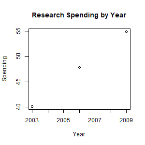
   1. Create a scatterplot of Spending vs. Year. Answer:
      

      > year <- c(2003, 2006, 2009)
      > spending <- c(40.1, 47.8, 54.9)
      > plot(year, spending, xlab="Year", ylab="Spending")
      

      
   2. Use R to obtain x, y, SD+_x, SD+_y, and r_xy Answer:
      

      > year
      [1] 2003 2006 2009
      > spending
      [1] 40.1 47.8 54.9
      > mean(year)
      [1] 2006
      > mean(spending)
      [1] 47.6
      > sd(year)
      [1] 3
      > sd(spending)
      [1] 7.402027
      > cor(year, spending)
      [1] 0.9997262
      

   3. Obtain the regression equation by hand using the statistics from Question 2b. When performing hand calculations, you can use R as a calculator. Verify your answer with the R lm function. Answer:
      The regression equation is
            y - y = (r * SD+_y / SD+_x)(x - x)
            y - 47.6 = (0.9997262 * 7.402027 / 3)(x - 2006)
            y - 47.6 = 2.466667 * (x - 2006)
            y = 2.466667 x - 2.466667 * 2006 + 47.6
            y = 2.466667 x - 4900.534
      To compute the regression equation using R, we first need to create a data frame containing the data. Then we use the lm function to obtain the regression model:
      

      > df <- data.frame(x=year, y=spending)
      > model <- lm(y ~ x, data=df)
      > print(model)
      
      Call:
      lm(formula = y ~ x, data = df)
      
      Coefficients:
      (Intercept) x 
      -4900.533 2.467 
      

   4. Compute the predicted values by hand. Check your answer using this R function call:
      

      > pred <- predict(model)
      

      Use the model obtained in Exercise 2c:
      y^{^}₁ = 2.467 * x₁ - 4900.533 = 2.466667 * 2003 - 4900.534 = 40.2
      y^{^}₂ = 2.467 * x₂ - 4900.533 = 2.466667 * 2006 - 4900.534 = 47.6
      y^{^}₃ = 2.467 * x₃ - 4900.533 = 2.466667 * 2009 - 4900.534 = 55
      We can perform this calculation in one line using R:
      

       > 2.466667 * c(2003, 2006, 2009) - 4900.534
      [1] 40.2 47.6 55.0

      Check your answer using the R predict function, which obtains the predicted values from the model:
      

      > p <- predict(model)
         1    2    3 
      40.2 47.6 55.0
      

   5. Compute the residuals, which are computed as e^{^}_i = y_i - y^{^}_i
            e^{^}₁ = y₁ - y^{^}₁ = 40.1 - 40.2 = -0.1
            e^{^}₂ = y₂ - y^{^}₁ = 47.8 - 47.6 = 0.2
            e^{^}₃ = y₃ - y^{^}₁ = 54.9 - 55.0 = -0.1
      Check your answer using the R resid function, which computes the residuals from the model. Answer:
      

      > resid(model)
         1   2    3 
      -0.1 0.2 -0.1 
      

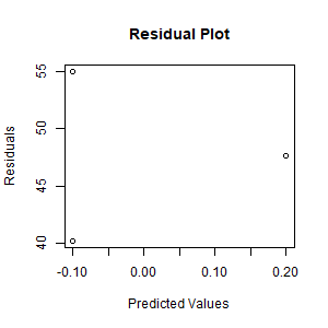
   6. Create the residual plot of residuals vs. predicted values. Answer:
      

      > plot(resid(model), predict(model), 
      + xlab="Predicted Values", ylab="Residuals", 
      + main="Residual Plot")
      

      
   7. Compute the normal scores by hand (n=3).
      Answer: the normal scores when n=3 divid the standard normal density into 4 equal areas or 25% each. The z-scores that do this are found at -0.67, 0.00, and 0.67. These can be found using the R qnorm function like this:
      

      > qnorm(c(0.25, 0.5, 0.75))
      [1] -0.6744898 0.0000000 0.6744898
      

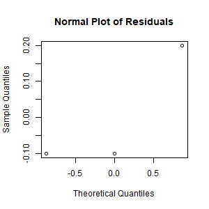
   8. Create and normal plot for the residuals. Answer:
      

      > qqnorm(resid(model), main="Normal Plot of Residuals")
      

      
2. What is the difference between the true regression equation and the estimated regression equation?
   Answer: recall the ideal measurement model: x_i = μ + e_i (actual measurement = true value + random error. μ is usually unknown and estimated by μ^{^}= x.
   
   The true regression equation is y_i = a * x_i + b, where the slope a and the intercept b are unknown and must be estimated by a^{^} and b^{^}, which are determined from the estimated regression equation:
         y - y = (r^{^} * SD+_y / SD+_x)(x - x)
   which is rewritten as
         y = a^{^} * x + b^{^}.

Project 3

• Look at the project description for Project 3 .

The Regression Fallacy

• During their flight training, Air Force pilots make two practice landings with their instructor. The pilots that make a good first landing tend to do worse on the second landing; the pilots that make a poor first landing do better on the second landing. Conclusion: criticism helps the pilots, whereas praise hurts them. Policy change: the supervisor of the flight instructors tells them to criticize all landings, good or bad. Is this policy change warrented?
• In fact, the criticism is not warrented. This is an example of the regression fallacy.
• Look at this graph of pre-test and post-test scores marked by the dots:
  
  
  
  The green line indicates where the dots would be if the pre and post scores were the same. The red line is the regression line, which shows where the pre-test score and its associated predicted post-test score would lie. As in the previous example of the Air Force pilots, a student with a high pre-test score is predicted to do worse on the post-test; a student with a low pre-test score is predicted to do better on the post-test.
• Practice Problem: Collect the following data for adult men: the subject's height, the height of the subject's father.
  
  1. Would you expect a person with a very tall father to be shorter or taller than his father?
     Answer: A very tall person is expected to be shorter than his father.
  2. Would you expect a person with a very short father to be shorter or taller than his father?
     Answer: A very short person is expected to be taller than his father.

Additional Regression Problem

We will work this problem in class on Monday, May 13.

• Root Mean Square Error
• A law school finds this relationship between LSAT scores (independent variable x) and first-year scores (dependent variable y). The data are bivariate normal. Here are the summary variables:
  x = 162    SD_x = 6
  y = 68    SD_y = 10
  r = 0.6
  
  1. About what percentage of the students have first-year scores over 75? Because the data are bivariate normal, the first-year scores are normally distributed, so you can use the normal table.
  2. Of those students who scored 165 on the LSAT, about what percentage have first-year scores over 75? Visualize these scores as lying in a thin vertical rectangle centered at LSAT = 165.