To Notes

IT 223 -- Apr 10, 2024

Review Problems

1. Show that the default for the R histogram hist function is right-inclusive bins. Show how to make the hist function use left-inclusive bins.
   Answer: Use R to define the dataset vector x and the vector of breakpoints for the histogram:
   

   > x <- c(0.5, 0.5, 0.5, 1, 1.5, 1.5, 1.5)
   > x
   [1] 0.5 0.5 0.5 1.0 1.5 1.5 1.5
   > b <- c(0, 1, 2)
   > b
   [1] 0 1 2
   

   Now create the histogram with bins 0 to 1 and 1 to 2 using the breakpoints vector c(0, 1, 2):
   

   > hist(x, breaks=b)
   

   Here is the histogram:
   
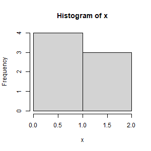
   This histogram shows that the data point 1 is included in the left bin, because the histogram bins are right inclusive: (0, 1], (1, 2]. To make the histogram bins left inclusive (like SPSS, SAS, Minitab, and Python, set the right argument to FALSE:
   

   hist(x, breaks=c(0, 1, 2), right=FALSE)
   

   Now this histogram is created:
   
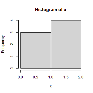
   This shows that the bins are [0, 1), [1, 2), which are left inclusive.
2. Show that when the histogram bins are all the same width, the height of the bars is the count or frequency in each bin. However, when the widths of the bins are not equal, the vertical axis represents a density, with the vertical axis being Percent per Horizontal Unit. In the second case, the area of the bar represents the percentage of observations in that bin.
   Answer: Create one histogram with equal bin widths: [0, 1], (1, 2], and another histogram with unequal bin widths:
   

   > x <- c(0.5, 0.5, 0.5, 1.5, 1.5)
   > b1 <- c(0, 1, 2)
   > b2 <- c(0, 1, 4)
   > hist(x, breaks=b1, main="Equal Width Bins")
   > hist(x, breaks=b2, main="Unequal Width Bins")
   

   The resulting histograms:
   
   
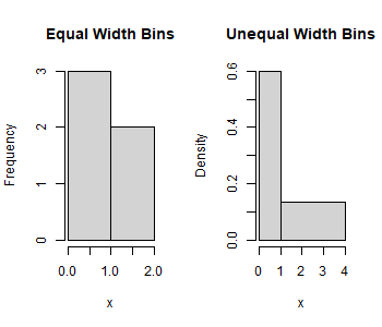
   For the Equal Width Bins histogram, the vertical axis label is Frequency and the vertical units are the counts in each bin; for the Unequal Bin Widths histogram, the vertical label is Density and the vertical units are fraction of observations per horizontal unit.
3. What is a critical point for a curve?
   Ans: A critical point of a curve is where the slope of the curve is horizontal For a normal curve, the x-value of the critical point is the center of the curve. The normal curve is symmetric around the center.
4. What is an inflection point for a curve?
   Answer: an inflection point of a curve is where the curve changes from concave down to concave up, or vice versa.
5. What is the sample mean?
   Answer: the sample mean is another name for the sample average. If x₁, x₂, ... , x_n is the dataset, the sample mean is the sum of the observations divided by the number of the observations:
          X = (x₁, x₂, ... , x_n) / n

Descriptive Statistics

• If a histogram (drawn without vertical bar lines) is bell-shaped or normal, it can be described by its center μ and spread σ:
  
  
• For a bell-shaped histogram, if the sample size n is large, the statistics x (sample average) and SD+ (sample standard deviation) are good estimates of μ and σ.
• x and SD+ form a parsimonious description of a bell-shaped histogram.
• The sample average is also called the sample mean.
• Estimates of the Center of a Dataset: Mean   Median   Trimmed Mean
• Estimators of the Spread of a Dataset: SD   SD⁺   MAD

Practice Problems

1. What happens to x and Q2 for a dataset
   
   1. if every observation is increased by 7?
      Ans: Both x and Q2 are increased by 7.
      x_new = (x₁ + 7 + ... + x_n + 7) / n
             = (x₁ + ... + x_n) / n + (7 + ... + 7) / n
             = x + (1/n) 7 / n = x + 7
   2. if every observation is multiplied by 3?
      Ans: Both x and Q2 are multiplied by 3.
      x_new = (3x₁ + ... + 3x_n) / n
             =  3(x₁ + ... + x_n) / n = 3 x
   3. if the largest observation is increased by 1000?
      Ans: The mean is increased by 1000 / n, the median is unchanged if n ≥ 3.
      (1/n)(x₁ + ... + (x_n + 1000)) = x + 1000 / n
2. What happens to SD for a dataset if
   
   1. if every observation is increased by 7?
   2. if every observation is multiplied by 3?
3. Show that the mean is the center of gravity of the dataset.
   Ans: In class we balanced a cardboard histogram on a pencil and showed that the center of gravity is the point on the x-axis where the histogram balances (does not tip to the left or right. Here is the algebraic demonstration: m is the point where the histogram balances, and x₁ - m is the turning moment that tries to turn the histogram to the left or right. A negative moment tries to tip the histogram to the left; a positive moment tries to top the histogram to the right. We want the moments to sum to zero so that the histogram balances.
   (x₁ - m) + ... + (x_n - m) = 0
   (1/n)[(x₁ - m) + ... + (x_n - m)] = 0
   (1/n)(x₁ + ... + x_nm) - (1/n) n m = 0
   x - m = 0, so m = x.
4. Compute the 20%-trimmed mean of this dataset:
          1   7   4   6   94   5   5   7   3   6
   Ans: Trimming 10% of the variables off of the bottom and 10% off of the top, means omitting 1 and 94. The average of the remaining variables is 5.375.
   Perform this calculation using R. If x is the complete dataset,
   

   > mean(x, trim=0.05)
   

   where trim=0.05 means trim 0.05 of the observations from the left and 0.05 of the observations from the right.
5. Without doing any calculations, compute the SD of this dataset:
        4   4   4   4   4
6. Without doing any calculations, compute the SD of this dataset:
         0   0   0   0   10   10   10   10
7. Compute the MAD of this dataset:
        20    10    15    15

Comparison of Mean and Median

1. The mean of a dataset is its center of gravity.
2. Find the center of gravity of a histogram cut out of cardboard.
3. The median divides a dataset in half.
4. If a histogram cut out of cardboard were cut at the median line, both of the resulting pieces would weigh the same.
5. The mean is affected more by changes in outliers than the median is affected.
6. The mean is pulled in the direction of the long tail of a skewed histogram, relative to the median.
7. Practice Problem: Compute the mean the histograms in Review Exercise 5 oF April 3 by using a weighted average of the midpoints of each rectangle weighted by the proportion of observations represented by that rectangle.

The Ideal Measurement Model

• No measurement is perfect.
• Every measurement involves some random error and systematic bias.
• The ideal measurement model assumes that a set of measurements has no systematic bias, and that the random errors are independent with the same standard deviation everywhere (homoscedastic).
• More details on the Ideal Measurement Model.

Analyze the NBS-10 Dataset

• Use R to obtain the following for the NIST-10 and PaperThickness datasets:
  
  1. x and SD+
  2. Histograms with three different bin widths
  3. Outliers using the boxplot
  4. z-scores
  5. Outliers using z-scores
  6. Standard error of the average
  7. Boxplot after removing outliers (according to first boxplot).
• Warning: do not automatically delete the outliers from the dataset. They may be the most important observations in the dataset.
• Here is a story (that might be an urban legend) about deleting outliers. Climatologists were studying the ozone levels in the upper atmosphere at the South Pole. In the 1960s, it was common for engineers to routinely delete outliers from the dataset, suspecting that they were bad observations. One of the data analysts therefore was deleting outliers from the Ozone observations dataset. Because of this, the hole in the ozone layer at the South pole was discovered several years later than it should have been.

Project 2

• Go over Project 2a.

The Normal Distribution

The Standard Error of the Average