To Documents

The Normal Distribution

Introduction

• A univariate dataset that has an approximately bell-shaped histogram is said to have a normal distribution.
• Here some examples of datasets that have approximately normal distributions:
  Heights of living things, weights of living things, lengths of inert appendages (hair, claws, nails, teeth) of biological specimens in the direction of growth, blood pressure of adult humans of fixed gender, velocities of molecules in an ideal gas, measurement errors, IQ scores, SAT scores.
  In finance, changes in the logarithm of exchange rates, price indices, and stock market indices are assumed normal in the Black-Scholes Model. The logarithm is used in the Black-Scholes model because these values behave like compound interest and so are multiplicative.
• Abraham DeMoivre was the first to write down the equation for the a normal histogram with center μ = 0 and spread σ = 1:
   
       p(x) = (1 / √(2π)) exp(-0.5x²) = 0.39894 * 2.71828 ^ (-0.5x²)
   
  Recall that π = 3.14159 and e = 2.71828.
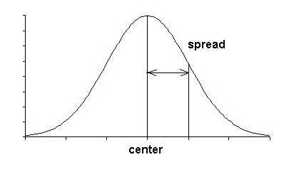
• Use R to plot the normal curve for the z values from -4 to 4 by 0.1
• If x and SD really a parsimonious description of a histogram, then given x and SD, we should be able to reconstruct the histogram; that is, we should be able to predict the proportion of observations in any bin of the form (-∞, a], (a, ∞], or [a, b].
• We start with the simplest case of a normal histogram with center 0 and spread 1.
   
  
• Our tool for finding areas under the normal curve is the standard normal table.
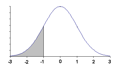
• Example 1:   What proportion of the observations are in this bin: (-∞, -1.00]?
   
  
   
  Solution: The value -1.00 on the x-axis of the normal curve is called a z-value. Use the first table in the normal table for negative numbers. Look in the -1.0 row and the .00 column to find .1587. The answer is: 0.1587.
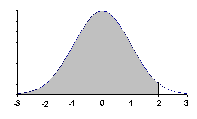
• Example 2:   What proportion of the observations are in this bin: (-∞, 2.00]?
   
  
   
  Solution: Look the z-value 2.00 up in the second table for positive numbers, also in the standard normal table. Look in the 2.0 row and the 0.00 column to find .9772. The answer is 0.9772.
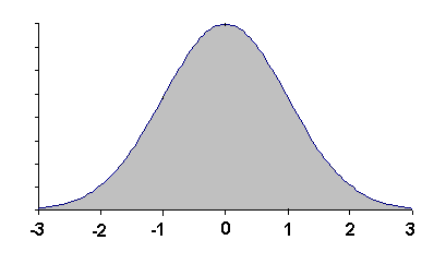
• Example 3:   What proportion of the observations are in this bin: (-3.00, 3.00]?
   
  
   
  Solution: (-3.00, 2.00] can be written as the set-theoretic difference (-∞, 2.00] - (-∞, -3.00]. Look up these bins in the normal table: (-∞, 2.00] has the proportion 0.9987 and (-∞, -3.00] has the proportion 0.0013. Therefore the proportion of observations in (-3.00, 2.00] = area (-∞, 2.00] - area (-∞,  -3.00] is 0.9987 - 0.0013 = 0.9974.
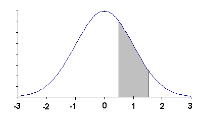
• Note: is does not matter whether we ask for the proportion of observations in (-3.00, 2.00], (-3.00, 2.00), [-3.00, 2.00), or [-3.00, 2.00]. They contain the same proportion of observations because the normal curve is an idealized continuous histogram where the the proportion of observations at a single point is always zero.
• Example 4:   What proportion of the observations are in this bin: (1.5, 2.5]?
   
  
   
  Solution: area (1.50, 2.50] = area (-∞, 2.50] - area (-∞, 1.50]. The the normal table gives the proportion of observations as 0.9938 - 0.9332 = 0.0606.
• In the case where the normal histogram is not standard, any intervals must be first converted to standard units by subtracting off the mean and then dividing by the standard deviation.
• The values converted to standard units are called z-scores.
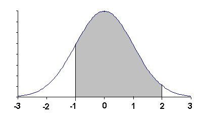
• Example 5: If the mean is 50 and the standard deviation is 10, what proportion of the observations are between 40 and 70?
  Solution: Convert 40 and 70 to z-scores:
   
      z = (x - μ) / σ = (40 - 50) / 10 = -1
   
  and
   
      z = (x - μ) / σ = (70 - 50) / 10 = 2
   
  Then the proportion of observations in the bin (-1, 2] = area (-∞, 2] - area (-∞, -1] is 0.9772 - 0.1587 = 0.8185.