IT 223 -- Mar 9, 2026

IT 223 -- Mar 9 , 2026

Review Exercises

Practice Problems for t-tests

Psychology experiments involve testing the ability of rate to navigate mazes. The mazes are classified according to difficulty, as measured by the average length of time it takes rats to find the food at the end. One researcher needs a maze that will take rats an average of about one minute to solve. He tests one maze on several rats, collecting this data

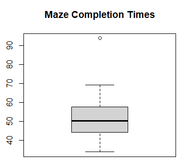
38.4 57.6 46.2 55.5 62.5 49.5 38.0 
40.9 62.8 44.3 33.9 93.8 50.4 47.9
35.0 69.2 52.8 46.2 60.1 56.3 55.1

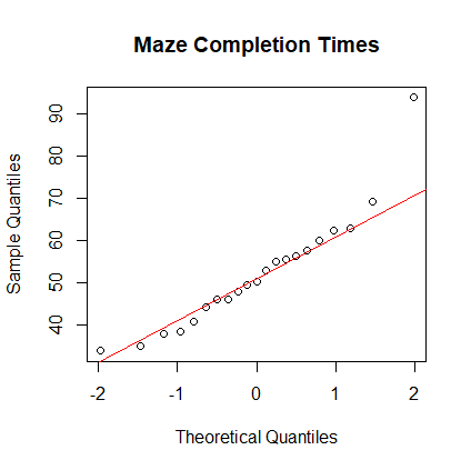
Form the normal plot and box plot of the maze times. Are the times normally distributed? Answer:

> times <- scan( )
1: 38.4 57.6 46.2 55.5 62.5 49.5 38.0 
8: 40.9 62.8 44.3 33.9 93.8 50.4 47.9
15: 35.0 69.2 52.8 46.2 60.1 56.3 55.1
22: 
Read 21 items
> boxplot(times, main="Maze Completion Times")
> qqnorm(times, main="Maze Completion Times")
> qqline(times, col="red")

Test the hypothesis that the true completion time is one minute. Answer:

        One Sample t-test

data:  times
t = -2.6319, df = 20, p-value = 0.01598
alternative hypothesis: true mean is not equal to 60
95 percent confidence interval:
 46.03498 58.38406
sample estimates:
mean of x 
 52.20952

The p-value is less than 0.05 so reject the null hypothesis that the true time to complete the maze is 60 seconds.

Eliminate the outlier and perform the hypothesis test again.
Answer: the outlier is 93.8 at index 12, which we can delete like this:

> # Indices with negative values mean
> # delete the value at that index.
> times <- times[-12]
> # Perform t-test again:
> t.test(times, mu=60)

        One Sample t-test

data:  times
t = -4.4568, df = 19, p-value = 0.0002705
alternative hypothesis: true mean is not equal to 60
95 percent confidence interval:
 45.49475 54.76525
sample estimates:
mean of x 
    50.13

The p-value = 0.0002705 is much smaller after deleting the outlier because the standard deviation of the times is smaller.

A food company marks the net weight of their potato chip bags as 28.3 grams. To test whether this claim is true, students collect and measure the net weights of bags. Here is the dataset
```
29.3  28.2  29.1  28.7  28.9  28.5
```
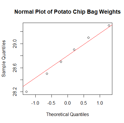
1. Form the normal plot of the new weights of the potato chip bags. Are the weights normally distributed? Answer:
```
> weights <- scan( )
1: 29.3 28.2 29.1 28.7 28.9 28.5
7: 
Read 6 items
> qqnorm(weights)
> qqline(weights, col="red")
```
2. Test the hypothesis that the true weight of potato chip bags is 28.3 grams. Answer:
```
 > t.test(weights, mu=28.3)
 
        One Sample t-test

data:  weights
t = 2.9445, df = 5, p-value = 0.03209
alternative hypothesis: true mean is not equal to 28.3
95 percent confidence interval:
 28.36138 29.20529
sample estimates:
mean of x 
 28.78333 
```
  The p-value is less than 0.03209 so reject the null hypothesis.

The Paired Sample t-test

Goal: to test whether there is a significant difference in measurements between subjects from two different groups.
Typically, one group is the treatment group and the other group is the control group.
For the paired sample t-test, each subject in one group is matched with a subject in the other group.
Then compute the differences in the response variable and perform a one-sample t-test on the differences.
For each of these scenarios, which which type of two-sample t-test should be used: paired or independent?
1. Comparing blood pressures of patients before and after taking a medication.
  Answer: paired two-sample t-test
2. Comparing average salaries at companies A and B.
  Answer: independent two sample t-test
3. Comparing midterm and final scores in a class.
  Answer: paired two-sample t-test
4. Comparing the durability of two types of artificial hip joints.
  Answer: independent two sample t-test. You can't give two different hip joints to the same person.
5. Comparing the durability of two types of house paints.
  Answer: independent two sample t-test.
6. Comparing the vertical jump of basketball players that participate in a specific weight training program.
  Answer: paired two-sample t-test.
Example 1: To test whether a new type of shoe sole material (type B) is better than the old type (type A), manufacture 10 pair of shoes where one shoe is made of type A and the other of type B. Randomly assign the type of material to left or right. Here is the data:
```
SoleMaterialA: 13.2 8.2 10.9 14.3 10.7 6.6 9.5 10.8 8.8 13.3
SoleMaterialB: 14.0 8.8 11.2 14.2 11.8 6.4 9.8 11.3 9.3 13.6
```
Perform the paired-sample t-test to see if there is a real difference between the two sole materials, or if it is just chance variation.
Here are the five steps of the two-sample t-test:
1. Write down the null and alternative hypothesis:
  H₀: SoleMaterial A = SoleMaterial B
  H₁: SoleMaterial A ≠ SoleMaterial B
2. Obtain the test statistic from R: t = -3.349
3. Using the t-table, obtain a 95% confidence interval with n - 1 = 10 - 1 = 9 degrees of freedom:
  I = [-2.26, 2.26]
4. t ∉ I so reject H₀.
5. Find the p-value from the R output: p = 0.009.
The test statistic for the two-sample t-test can be obtained by computing the differences
diff = SolematerialA - SoleMaterialB,
then use R to perform a one-sample t-test on the variable diff.
Here are the five steps of the one-sample t-test performed with the diff variable:
1. Write down the null and alternative hypothesis:
  H₀: diff = 0
  H₁: diff ≠ 0
2. Obtain the test statistic from R: t = -3.349
3. Using the t-table, obtain a 95% confidence interval with n - 1 = 10 - 1 = 9 degrees of freedom:
  I = [-2.26, 2.26]
4. t ∉ I so reject H₀.
5. Find the p-value from the R output:
  p = 0.009.
Notice that the test statistic t and the p-value are exactly the same whether a paired two-sample t-test is performed or whether a one-sample t-test on the differences is performed.

The Independent Two-Sample t-test

With the independent sample t-test, there is no pairing between between the subjects in the two groups.
To perform an independent two-sample t-test put all the values of the response variable in one column and in a second column, values marking the groups the subjects are in.
Example 3: Here is the Shoes data of Example 5:
```
SoleMaterialA: 13.2 8.2 10.9 14.3 10.7 6.6 9.5 10.8 8.8 13.3
SoleMaterialB: 14.0 8.8 11.2 14.2 11.8 6.4 9.8 11.3 9.3 13.6
```
Load this data into the two data vectors materialA and materialB. Then perform an independent two-sample t-test with R.
```
> t.test(materialA, materialB, var.equal=TRUE)
```
This test uses the test statistic
.
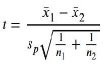where the pooled standard deviation s_p is defined by
.

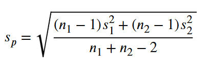An alternative to the independent two-sample t-test assuming equal variances for the two groups is the Welch test that does not assume equal variances. Using R, the test can be conducted like this:
```
> t.test(materialA, materialB, var.equal=FALSE)
```
Computational details are not shown here, but here is the R output:
```
        Welch Two Sample t-test

data:  materialA and materialB
t = -0.36891, df = 17.987, p-value = 0.7165
alternative hypothesis: true difference in means is not equal to 0
95 percent confidence interval:
 -2.745046  1.925046
sample estimates:
mean of x mean of y 
    10.63     11.04 
```
For this independent two-sample t-test, the result is not significant because p = 0.7165. The variability is greatly increased because we are ignoring the pairing between the two groups.

Example 4. A researcher wants to know if there is a difference in how busy someone is based on whether that person identifies as an early bird or a night owl. The researcher gathers data from people in each group, coding the data so that higher scores represent higher levels of being busy, and tests for a difference between the two at the 5% level of significance. Here is the dataset:

Early Bird: 23 28 27 33 26 30 22 25 26
Night Owl:  26 10 20 19 26 18 12 25

We name the two data vectors morning and night.

> morning <- scan( )
1: 23 28 27 33 26 30 22 25 26
10: 
Read 9 items
> night <- scan( )
1: 26 10 20 19 26 18 12 25
9: 
Read 8 items
> sd(morning)
[1] 3.391165
> sd(night)
[1] 6.141196
> boxplot(morning, night, names=c("morning", "night"),
+ main="Boxplots for the Two Groups")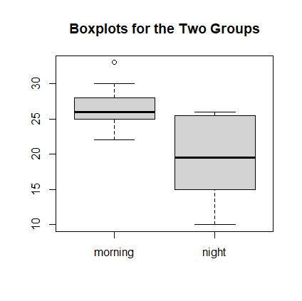

Here is the R output for the Welch Independent Two-sample t-test:

> t.test(morning, night, paired=FALSE, var.equal=FALSE)

        Welch Two Sample t-test

data:  morning and night
t = 2.9277, df = 10.626, p-value = 0.01422
alternative hypothesis: true difference in means is not equal to 0
95 percent confidence interval:
  1.755705 12.577629
sample estimates:
mean of x mean of y 
 26.66667  19.50000

Since the p-value is less than 0.05, we conclude that the difference of the group means is significantly different.

Inference for Simple Linear Regression

Question: if y = ax + b is the regression equation, what is the difference between a, b and a^{^}, b^{^}?
Example 5: The data file chem-reaction.txt contains two columns: (a) mass, the mass of the chemical used in the chemical reaction and (b) time, the time needed for the reaction to occur.
1. Create the scatter plot of time vs. mass. Answer:
```
> setwd("c:/workspace")
> df1 <- read.csv("chem-reaction.txt")
> print(df1)
mass time
1 5 40
2 7 120
3 12 180
4 16 210
5 20 240
> plot(df1$mass, df1$time, xlab="Mass (grams)", ylab="Time (sec)",
+ main="Reaction Time vs. Mass")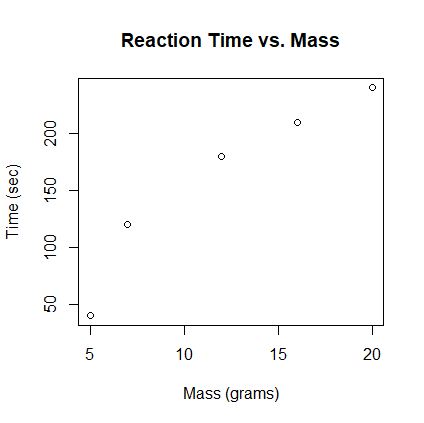
```
2. Find the linear regression equation for predicting time from mass. Answer:
```
> model1 <- lm(time ~ mass, data=df1)
> summary(model1)

Call:
lm(formula = time ~ mass, data = df1)

Residuals:
      1       2       3       4       5 
-32.545  23.039  22.000   3.169 -15.662 

Coefficients:
            Estimate Std. Error t value Pr(>|t|)  
(Intercept)   11.506     29.687   0.388   0.7242  
mass          12.208      2.245   5.437   0.0122 *
---
Signif. codes:  0 ‘***’ 0.001 ‘**’ 0.01 ‘*’ 0.05 ‘.’ 0.1 ‘ ’ 1

Residual standard error: 27.86 on 3 degrees of freedom
Multiple R-squared:  0.9079,    Adjusted R-squared:  0.8771 
F-statistic: 29.56 on 1 and 3 DF,  p-value: 0.01222
```
  The regression equation is time = 12.208 * 11.506.
3. Find the R-squared value for this equation. Interpret it.
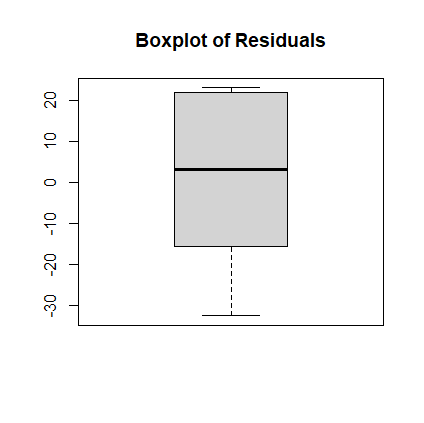
  Answer: the R-squared value is marked as Multiple R-squared in the R regression summary. It is 0.9079, which is the variation in the time variable that can be explained by the variation in mass.
4. Create the boxplot of the residuals.
```
> r <- resid(model1)
> boxplot(r, main="Boxplot of Residuals")
```
5. Create the scatterplot of the residuals vs. the predicted values. Interpret it. Answer:
```
> r <- resid(model1)
> p <- predict(model1)
> plot(p, r, xlab="Predicted Values", 
+ ylab="Residuals", main="Residual Plot")
```
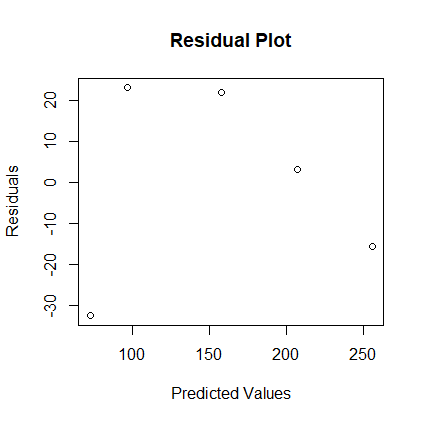
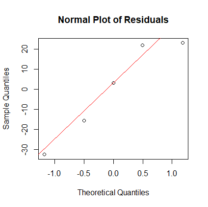
  The residuals appear to be biased, but since R² is so high, we don't worry about biased residuals too much.
6. Create the normal plot of the residuals. Interpret it. Answer:
```
> qqnorm(r, main="Normal Plot of Residuals")
> qqline(r, col="red") 
```
7. If y = ax + b is the true regression equation. Perform a t-test that tests the null hypothesis that the true value of the slope a is 0.
8. If y = ax + b. Perform a t-test that tests the null hypothesis that the true value of the intercept b is 0.
9. The the chemical reaction studied in this example, if the mass is 10.0, what is the predicted time for the chemical reaction?
Example 6: the blood alchohol level for a random sample of college students is tested after they drink a few beers. The data file beer-bac.txt contains two columns: (a) the number of beers (beers) consumed and (b) their blood alchohol levels (bac) after they drink the beers. Analyze the regression model and graphs of the resulting data. Use the output and graphs produced from this R script: beer-bac.R
1. Create the scatter plot of bac vs. beers.
2. Find the linear regression equation for predicting bac from beers.
3. Find the R-squared value for this equation. Interpret it.
4. Create the boxplot of the residuals.
5. Create the scatterplot of the residuals vs. the predicted values. Interpret it.
6. Create the normal plot of the residuals. Interpret it.
7. If y = ax + b. Perform a t-test that tests the null hypothesis that the true value of the slope a is 0.
8. If y = ax + b. Perform a t-test that tests the null hypothesis that the true value of the intercept b is 0.
9. The the chemical reaction studied in this example, if the number of beers consumed is 4, what is the predicted time for the chemical reaction?

The Pendulum Data

Take a pendulum consisting of a nut, thread, and paper that indicates the length of the pendulum in inches. Measure the time in seconds that it takes the pendulum to complete 15 complete periods.
Use your phone stopwatch to measure the time for 15 periods. Record your time to the nearest hundredth of a second.
Here is the pendulum data collected: pendulum.txt. The fields are LengthIn (length of pendulum in inches) and TimeFor15 (time for 15 periods of the pendulum).

Use R to convert the length to meters and find the period lengths:

> setwd("c:/workspace")
> # Read data frame from input file.
> df <- read.csv("pendulum.txt")
> print(df)
   LengthIn TimeFor15
1         5     10.87
2        10     15.42
3        15     18.66
4        20     21.65
5        25     24.21
6        30     26.60
7        35     28.14
8        40     29.99
9        45     32.34
10       50     33.61
> # Convert length in inches to meters
> # There are 2.54 cm per inch
> and 0.01 m per cm.
> len <- df$LengthIn * 2.54 * 0.01
> print(len)
 [1] 0.127 0.254 0.381 0.508 0.635 0.762 
 [7] 0.889 1.016 1.143 1.270
> # Divide by 15 to obtain time for one period in sec.
> per <- df$TimeFor15 / 15
> print(per)
 [1] 0.7246667 1.0280000 1.2440000 1.4433333 
 [5] 1.6140000 1.7733333 1.8760000 1.9993333
 [9] 2.1560000 2.2406667

Using R, obtain these two regression models: (1) predict per from len and (2) predict per from sqrtlen (square root of length)
1. Independent variable: Length in meters (len); Dependent variable: Period (per)
  Answer: use R to construct the regression model per ~ len:
```
model1 <- lm(per ~ len)
> summary(model1)

Call:
lm(formula = per ~ len)

Residuals:
Min 1Q Median 3Q Max 
-0.155067 -0.020467 0.004333 0.067533 0.085200 

Coefficients:
Estimate Std. Error t value Pr(>|t|) 
(Intercept) 0.71747 0.05761 12.45 1.61e-06 ***
len 1.27769 0.07311 17.48 1.17e-07 ***
---
Signif. codes: 0 ‘***’ 0.001 ‘**’ 0.01 ‘*’ 0.05 ‘.’ 0.1 ‘ ’ 1

Residual standard error: 0.08433 on 8 degrees of freedom
Multiple R-squared: 0.9745, Adjusted R-squared: 0.9713 
F-statistic: 305.4 on 1 and 8 DF, p-value: 1.172e-07
```
  The R-squared value is 0.9745, which is very good. However, we can do better. The plot of per vs. len shows a curvilinear relationship between these variables. Furthermore, the physics formula below shows that √L (sqrtlen = square root of len) is a better independent variable to use for predicting period.
2. Independent variable: Length in meters (len); Dependent variable: Square Root of Period (sqrt(per))
The physics formula for predicting period from length for a pendulum is
per = 2π √len / g
where π = 3.14159 and g = 9.81 meters per second squared.
Answer: use R to construct the regression model per ~ sqrtlen.
```
> sqrtlen <- sqrt(len)
> model2 <- lm(per ~ sqrtlen)
> summary(model2)

Call:
lm(formula = per ~ sqrtlen)

Residuals:
       Min         1Q     Median         3Q        Max 
-0.0189833 -0.0114976 -0.0008825  0.0103954  0.0210963 

Coefficients:
            Estimate Std. Error t value Pr(>|t|)    
(Intercept)  0.03227    0.01631   1.979   0.0832 .  
sqrtlen      1.97034    0.01951 100.975 1.03e-13 ***
---
Signif. codes:  0 ‘***’ 0.001 ‘**’ 0.01 ‘*’ 0.05 ‘.’ 0.1 ‘ ’ 1

Residual standard error: 0.01478 on 8 degrees of freedom
Multiple R-squared:  0.9992,    Adjusted R-squared:  0.9991 
F-statistic: 1.02e+04 on 1 and 8 DF,  p-value: 1.033e-13
```
The R² value for Model 2 is 0.9992, which is better than the R² = 0.9745 from Model 1. Rewrite the physics formula for predicting period from length like this:
     per = 2π √len / g = (2π / √g) * √len + 0 = a * sqrtlen + b.
Let's compare the coefficients a and b obtained from the R regression model2 summary with the values from the physics formula:

Physics model2

a = 2*pi/sqrt(g) = 2.006 1.97034

b = 0 0.03227

Since the summary of model2 shows the standard errors of the estimated regression coefficients a^ and b^, shown in the model2 column, we can compute confidence intervals for their true values, shown in the Physics column of the table:
     -t_0.025,10-2 ≤ (a^ - a) / SE_a^ ≤ t_0.025,10-2
     -2.306004 ≤ (1.97034 - a) / 0.01951 ≤ 2.306004
     -2.306004 * 0.01951 - 1.97034 ≤ - a ≤ 2.306004 * 0.01951 - 1.97034
    - 2.01533 ≤ -a ≤ -1.92535
      2.01533 ≥ a ≥ 1.92535
Thus a 95% confidence interval for the true regression coefficient a is (1.925, 2.015). In fact a = 2.006, from the Physics column of the table above. This value of a does belong to this confidence interval.

Note: the degrees of freedom to use when looking up the value -t_0.025,10-2 in the t-table is n - 2. We loose two degrees of freedom for estimating a and b with a^ and b^, just like we lost one degree of freedom in the one sample t-test by estimating μ with x.

Similarly, we can compute a 95% confidence interval for the true value of the regression coefficient b = 0:
      t_0.025,10-2 ≤ (b^ - b) / SE_b^ ≤ t_0.025,10-2
      -2.306004 ≤ (0.03227 - b) / 0.01631 ≤ 2.306004
      -2.306004 * 0.01631 - 0.03227 ≤ -b ≤ 2.306004 * 0.01631 - 0.03227
      -0.06988093 ≤ -b ≤ 0.005340925
      0.06988093 ≥ b ≥ -0.005340925
Thus a 95% confidence interval for b is (-0.00534, 0.0699). If fact b = 0 from the Physics column of the table above. The value of b does belong to this confidence interval.

Physics	model2
a = 2*pi/sqrt(g) = 2.006	1.97034
b = 0	0.03227