May 4, 2026

To Notes

IT 223 -- May 4 , 2026

Review Exercises

If X is a random variable with expected value E(X), variance Var(X), and standard deviation σ_X, use the formulas that you know to obtain the following:
      E(S)   Var(S)   σ_S    z_S
      E(X) Var(X)   σ_X    z_X
Assume that S = x₁ + x₂ + ... + x_n and X, where the x_i are all independent.
Answer:
      E(S) = E(X₁)
      Var(S) = n * Var(X₁) if X₁, ... , X_n are independent.
      σ_S = √n * σ_X1 if X₁, ... , X_n are independent
      z = (S - E(S) ) / σ_S
      E(X) = E(X₁)
      Var(X) = E(X₁) / n, if X₁, ... , X_n are independent.
      σ_X = σ_X1 / √n
      z = (X - E(X)) / σ_X
What is a confidence interval?
Answer: a 95% confidence interval is expected to contain the unknown parameter, for example μ, 95% of the time if the expected value of the sample mean is equal to μ.
What is a statistical test?
Answer: it is a test to see if a sample statistic (e.g., the sample mean x) is equal to a population parameter (e.g., the population mean). We write this as H₀: x = μ. Here are the five steps of a z- or t-test:
1. Write down the null hypothesis and the alternative hypothesis.
2. Compute the value of the test statistic z or t.
3. Find a 95% (or 99%) confidence interval I for z or t using the z- or t-tables.
4. If z or t ∈ I, accept H₀; if z or t ∉ I, reject H₀.
5. Compute the p-value that, which is the probability of obtaining a test statistic as extreme or more extreme as the value actually obtained, given that the null hypothesis is true.
For a standard normal z-score, verify these probabilities using R:

z P(-1 ≤ z ≤ 1)

(-1, 1)         0.68

(-2, 2)         0.95

(-3, 3)         0.997

Answer:
```
> pnorm(1) - pnorm(-1)
[1] 0.6826895
> pnorm(2) - pnorm(-2)
[1] 0.9544997
> pnorm(3) - pnorm(-3)
[1] 0.9973002
```
Use the R function qnorm to verify that a 95% confidence interval for standard normal z-score is [-1.96, 1.96]. Also verify that a 99% confidence interval for such a z-score is [-2.58, 2.58].
Answer: for a 95% confidence interval, the area in the two tails is 100% - 95% = 5% and the area of one tail is 5% / 2 = 2.5% = 0.025. Using R:
```
> qnorm(0.025)
[1] -1.959964
```
For a 99% confidence interval, the area of the two tails is 100% - 99% = 1% and area in one tail is 1% / 2 = 0.5% = 0.005. Using R:
```
> qnorm(0.005)
[1] -2.575829
```
How is the t-test different than the z-test?
Answer: for a z-test, n ≥ 30, so even though the random variable x is not normally distributed, the average x is approximately normally distributed by the Central Limit Theorem. Thus we can use the normal table to find confidence intervals for z-tests.

For a t-test, we do not assume that n > 30, so for a good result, the original data should be approximately normsl. Create a normal plot of the data to check this. Since n is small, the sample standard deviation s_x may not be a good approximation of the population standard deviation σ_x. Therefore we need a wider confidence interval to account for this extra uncertainty. For example, a 95% confidence interval for the z-test is (-1.96, 1.96), but a 95% confidence interval for a t-test with n = 5 is wider: (-2.78, 2.78).
What are degrees of freedom? Why are they important for the t-test?
Answer: when computing the sample standard deviation, the sum of the deviations x_i is always zero. These lines show why:
(x₁ - x) + (x₂ - x) + ... + (x_n - x) =
(x₁ + x₂ + ... + x_n) - (x + x + ... + x) = nx - nx = 0
Because the sum of the deviations is zero, once n - 1 deviations have been computed, the nth deviation has been already determined. This is why we say that there are only n - 1 degrees of freedom for the deviations.
How is the significance level for a test related to the confidence interval for the test statistic?
Answer: if a confidence interval for a test is 0.95, the test's significance level is 1 - 0.95 = 0.05. In general, if the significance level of a test is α, the significance level of the test is 1 - α.
Who invented the t-test?
Answer: William Gosset (1876 - 1937) invented the t-test to control the quality when brewing beer at the Guinness Company outside of Dublin Ireland. Guinness did not allow employees to publish their research because it was proprietary. Gosset published his research about the t-test using the pen name Student. Even today, the t-test is often called the Student's t-test.
Use R to perform the t-test for the CO Concentration Example from Mar 2. Answer:
```
> t.test(conc, mu=70)

        One Sample t-test

data:  conc
t = 2.16, df = 4, p-value = 0.09689
alternative hypothesis: true mean is not equal to 70
95 percent confidence interval:
 67.774 87.826
sample estimates:
mean of x 
     77.8 
```
Conclusion: because p = 0.09689 ≥ 0.05, reject the null hypothesis. There is not enough evidence to reject the null hypothesis.
Additionally,
1. Use the t-table to compute the 0.95 confidence interval for the t statistic.
  Answer: in the t-table, look in the Degrees of Freedom row 5 - 1 = 4 and the Upper Tail Probability column 0.025. The entry is 2.776.
2. Verify the 95% confidence interval for x in the R t-test output by solving this inequality:
        -t_0.025,df ≤ t ≤ t_0.025,df
  where
        t = (x - μ) / (s_x / √n)
  Answer: n = 5,   x = 77.8, s_x = 8.074652, so
  t = (x - μ) / (sd_x / √n) = (77.8 - μ) / (8.074652 / √5) = (77.8 - μ) / 3.611094
  Therefore the confidence interval is
  -2.776 ≤ t ≤ 2.776
  -2.776 ≤ (77.8 - μ) / 3.611094 ≤ 2.776
  -2.776 * 3.611094 ≤ 77.8 - μ ≤ 2.776 * 3.611094
  -2.776 * 3.611094 - 77.8 ≤ -μ ≤ 2.776 * 3.611094 - 77.8
  -87.83 ≤ -μ ≤ -67.77
  67.77 ≤ μ ≤ 87.83
  so (67.77, 87.83) is the 95% confidence interval for μ. This matches the confidence interval output by the t.test function.
Perform a t-test to determine if student test scores in a class differ from the national average of 75. These are the test scores:
```
 78  82  71  75  80  72  79  74  77  76
```
Perform the calculations "by hand" using R. Then verify your work using the R t.test function. Also use the t.test function at the 0.99 confidence level.

z	P(-1 ≤ z ≤ 1)
(-1, 1)	0.68
(-2, 2)	0.95
(-3, 3)	0.997

Practice Problems for t-tests

In 1998, as an adverting campaign, a cookie company claimed that every 18-ounce bag contained an an average of 1000 chocolate chips. Students at the Air Force Academy in Colorado Springs bought some randomly selected bags of cookies and counted the chocolate chips. Here is the dataset
```
1219 1214 1087 1200 1419 1121 1235 1345
1244 1258 1356 1132 1191 1270 1295 1135
```
1. Form the normal plot of the chocolate chip counts. Are the counts normally distributed?
2. Perform a 99%-level test of hypothesis that the average chocolate chip count is 1000 per bag.
Psychology experiments involve testing the ability of rate to navigate mazes. The mazes are classified according to difficulty, as measured by the average length of time it takes rats to find the food at the end. One researcher needs a maze that will take rats an average of about one minute to solve. He tests one maze on several rats, collecting this data
```
38.4 57.6 46.2 55.5 62.5 49.5 38.0 
40.9 62.8 44.3 33.9 93.8 50.4 47.9
35.0 69.2 52.8 46.2 60.1 56.3 55.1	
```
1. Form the normal plot and box plot of the maze times. Are the times normally distributed?
2. Test the hypothesis that the true completion time is one minute.
3. Eliminate the outlier and perform the hypothesis test again.
A food company marks the net weight of their potato chip bags as 28.3 grams. To test whether this claim is true, students collect and measure the net weights of bags. Here is the dataset
```
29.3  28.2  29.1  28.7  28.9  28.5.
```
1. Form the normal plot of the new weights of the potato chip bags. Are the weights normally distributed?
2. Test the hypothesis that the true weight of potato chip bags is 28.3 grams.

Normal Approximation for the Binomial Distribution.

Practice Problems:
1. Flip a fair coin 10,000 times. What is the probability of obtaining exactly 5,000 heads.
  Answer: use the normal approximation. By the Central Limit Theorem, the number of successes S for a Binomial experiment is close to normally distributed if the number of trials n is large. Find the probability that S is between 4999.5 and 5000.5. The standard error of S is
        σ_S = √n*p*(1-p) = √10000*0.5*(1-0.5) = 50
  The z scores are
        z_left = (4999.5 - 5000.0) / 50 = -0.001
  and
        z_right = (5000.5 - 5000.0) / 50 = 0.001
        P(z_left ≤ z ≤ z_right) = P(z ≤ z_right) - P(z ≤ z_left) = 0.007978713
  This probability can be computed directly using dbinom:
```
> dbinom(5000, 10000, 0.5)
[1] 0.007978646
```
  The two values 0.007978713 and 0.007978646 are not exactly the same, but the normal approximation is very good because n is large at 10,000.
2. Flip a fair coin 10,000 times. What is the probability of obtaining between 4,850 and 5,100 heads? Answer:
```
> # Calculate the probability of between
> # 4,850 and 5,100 successes out of 10,000 trials
> #
> # Normal approximation:
> pnorm(5100.5, mean=5000, sd=50) - 
+ pnorm(4849.5, mean=5000, sd=50)
[1] 0.9764782
>
> # Exact calculation with pbinom:
> pbinom(5100, size=10000, prob=0.5) - 
+ pbinom(4849, size=10000, prob=0.5)
[1] 0.9764817
```

The Paired Sample t-test

Goal: to test whether there is a significant difference in measurements between subjects from two different groups.
Typically, one group is the treatment group and the other group is the control group.
For the paired sample t-test, each subject in one group is matched with a subject in the other group.
Then compute the differences in the response variable and perform a one-sample t-test on the differences.
Example 1: To test whether a new type of shoe sole material (type B) is better than the old type (type A), manufacture 10 pair of shoes where one shoe is made of type A and the other of type B. Randomly assign the type of material to left or right. Here is the data:
```
SoleMaterialA: 13.2 8.2 10.9 14.3 10.7 6.6 9.5 10.8 8.8 13.3
SoleMaterialB: 14.0 8.8 11.2 14.2 11.8 6.4 9.8 11.3 9.3 13.6
```
Perform the paired-sample t-test to see if there is a real difference between the two sole materials, or if it is just chance variation.
Here are the five steps of the two-sample t-test:
1. Write down the null and alternative hypothesis:
  H₀: SoleMaterial A = SoleMaterial B
  H₁: SoleMaterial A ≠ SoleMaterial B
2. Obtain the test statistic from R: t = -3.349
3. Using the t-table, obtain a 95% confidence interval with n - 1 = 10 - 1 = 9 degrees of freedom:
  I = [-2.26, 2.26]
4. t ∉ I so reject H₀.
5. Find the p-value from the R output: p = 0.009.
The test statistic for the two-sample t-test can be obtained by computing the differences
diff = SolematerialA - SoleMaterialB,
then use R to perform a one-sample t-test on the variable diff.
Here are the five steps of the one-sample t-test performed with the diff variable:
1. Write down the null and alternative hypothesis:
  H₀: diff = 0
  H₁: diff ≠ 0
2. Obtain the test statistic from R: t = -3.349
3. Using the t-table, obtain a 95% confidence interval with n - 1 = 10 - 1 = 9 degrees of freedom:
  I = [-2.26, 2.26]
4. t ∉ I so reject H₀.
5. Find the p-value from the R output:
  p = 0.009.
Notice that the test statistic t and the p-value are exactly the same whether a paired two-sample t-test is performed or whether a one-sample t-test on the differences is performed.
Example 2. A company wants to evaluate a new training program for its sales team. They test 6 employees before the training and again after the training to see if there is a significant improvement in their scores. Here are the before and after scores:
```
Before: 70 80 75 85 90 70
After:  75 82 73 90 95 75
```

The Independent Two-Sample t-test

We will discuss this section again on May 9.

With the independent sample t-test, there is no pairing between between the subjects in the two groups.
To perform an independent two-sample t-test put all the values of the response variable in one column and in a second column, values marking the groups the subjects are in.
Example 3: Here is the Shoes data of Example 5:
```
SoleMaterialA: 13.2 8.2 10.9 14.3 10.7 6.6 9.5 10.8 8.8 13.3
SoleMaterialB: 14.0 8.8 11.2 14.2 11.8 6.4 9.8 11.3 9.3 13.6
```
Load this data into the two data vectors materialA and materialB. Then perform an independent two-sample t-test with R.
```
> t.test(materialA, materialB, var.equal=TRUE)
```
This test uses the test statistic
.
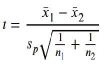where the pooled standard deviation s_p is defined by
.

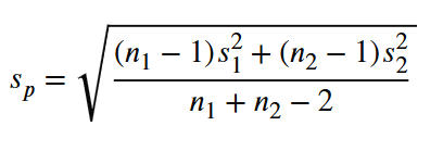An alternative to the independent two-sample t-test assuming equal variances for the two groups is the Welch test that does not assume equal variances. Using R, the test can be conducted like this:
```
> t.test(materialA, materialB, var.equal=FALSE)
```
Computational details are not shown here.
Example 4. A researcher wants to know if there is a difference in how busy someone is based on whether that person identifies as an early bird or a night owl. The researcher gathers data from people in each group, coding the data so that higher scores represent higher levels of being busy, and tests for a difference between the two at the 5% level of significance. Here is the dataset:
```
Early Bird: 23 28 27 33 26 30 22 25 26
Night Owl:  26 10 20 19 26 18 12 25
```