IT 223 -- Feb 4, 2026

Review Exercises

Find the expected normal scores for a dataset with n = 9.
Answer: find 9 z-values that divide the normal curve into 10 equal areas. To do this, use the standard normal tables to look up the z-scores that most closely correspond to these quantiles:
```
0.1  0.2  0.3  0.4  0.5  0.6  0.7  0.8  0.9
```
These z-scores are
```
-1.28 -0.84 -0.52 -0.25 -0.00 0.25 0.52 0.84 1.28
```

Use R to obtain the same z-scores (more accurately):

> qnorm(seq(0.1, 0.9, 0.1))
[1] -1.2815516 -0.8416212 -0.5244005 -0.2533471  0.0000000 
[6]  0.2533471  0.5244005  0.8416212  1.2815516

What does the correlation tell you about the relationship between two data vectors x and y?
Answer: the correlation of x and y tells you the amount of linear association between x and y.
Compute the correlation of x and y by hand:

Obs: 1 2 3 4 5

x: 1 2 3 4 5

y: 1 3 2 5 4

Verify your answer using R.
Answer:
x = (1 + 2 + 3 + 4 + 5) / 5 = 3,
x = (1 + 3 + 2 + 5 + 4) / 5 = 3,
SD_x = √((1-3)² + (2-3)² + (3-3)² + (4-3)² + (5-3)²) / 5) = √2
SD_y = √((1-3)² + (3-3)² + (2-3)² + (5-3)² + (4-3)²) / 5) = √2
Now compute the z-scores for both x and y:
z_xi = (x_i - x) / SD_x and z_yi = (y_i - y) / SD_y for i = 1, ... , n.
Then the correlation is the average of the products of the z-scores:
x_i      y_i        z_xi           z_yi       z_xi*z_yi
-----+-----+---------+---------+-----------
   1      1    -2/√2       -2/√(2)    +4/2 = 2
   2      3    -1/√2           0             0    = 0
   3      2        0        -1/√(2)       0    = 0
   4      5    +1/√2      +2/√(2)    +2/2 = 1
   5      4    +2/√2      +1/√(2)    +2/2 = 1
The average of the products is (2 + 0 + 0 + 1 + 1) / 5 = 0.8.
Verify your calculation with R:
```
> x <- 1:5
> x
[1] 1 2 3 4 5
> y <- c(1, 3, 2, 5, 4)
> y
[1] 1 3 2 5 4
> cor(x, y)
[1] 0.8 
```
Estimate the correlation r in these situations.
1. Height of father, height of son.
  i. -0.30 ii. 0.05 iii. 0.70 iv. 0.99
  Answer: 0.70
2. IQ of husband, IQ of wife.
  i. -0.70 ii. 0.00 iii. 0.60 iv. 1.00
  Answer: 0.60
3. Height of husband, height of wife if men always married women that were exactly 6 inches shorter.
  i. -0.60 ii. 0.60 iii. 0.99 iv. 1.00
  Answer: 1.00
4. Weight of husband, weight of wife if men always married women that weighed 70% of their weight.
  i. 0.00 ii. 0.50 iii. 0.70 iv. 1.00
  Answer: 1.00
Match the correlation to the dataset:
1. GPA in freshman year, GPA in sophomore year.
  i. 0.00 ii. 0.30 iii. 0.70 iv. 1.00
  Answer: 0.70
2. GPA in freshman year, GPA in senior year.
  i. 0.00 ii. 0.30 iii. 0.70 iv. 1.00
  Answer: 0.30
3. Length and weight of 2 by 4 boards.
  i. -0.50 ii. 0.005 iii. 0.30 iv. 0.70 v. 0.99
  Answer: 0.99
What would happen to the correlation r if
1. x were replaced by x + 10.
2. y were replaced by 2 * y + 8.
3. x and y were interchanged.
Answer: in all three cases, the correlation would remain the same.
How large must r be to be considered meaningful?
Answer: See the table in the Correlation document.

Linear Regression

With the laundry-detergent.txt dataset, use R to:

Load the data from the CSV dataset into the data vectors r (Rating) and p (Price).

> setwd("c:/workspace")
> getwd( )
[1] "c:/workspace"
> data_frame <- read.csv("laundry-detergent.txt")
> r <- data_frame$Rating
> p <- data_frame$Price
> r
[1]  61 55 50 46 35 32 59 52 48 46 34 29 56 51 
[15]  4  8 45 33 26 55 50 48 36 32 26
> p
[1]  17 30  9 13  8  5 22 23 16 13 12 14 22 11
[15] 15 17  7 11 16 15 18  8  6 13

Find the linear regression line for predicting Price from Rating.
```
> model <- lm(p ~ r)
> model

Call:
lm(formula = p ~ r)

Coefficients:
(Intercept) r 
-2.1443 0.3727 
```
The regression equation for predicting r from p is:
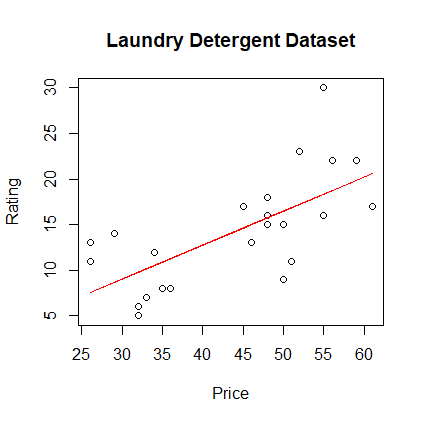
p = 0.3727 * r - 2.1443

Create a scatterplot of Price vs. Rating. Add the regression line to this plot:

> plot(r, p, xlab="Price", ylab="Rating", 
+ main="Laundry Detergent Dataset")
> pred <- predict(model)
> lines(r, pred, col="red")

Scatterplot for Laundry Detergent Dataset

Compute r and R².

> # Correlation between p and r
> cor(p, r)
[1] 0.6707535
> # R-squared value
> cor(p, r)^2
[1] 0.4499103

Create a residual plot (plot residuals vs. predicted values). Add the horizontal zero line.

> pred <- predict(model)
> lines(r, pred, col="red")
> res <- resid(model)
> plot(pred, res, xlab="Predicted Values", ylab="Residuals",
+ main="Laundry Detergent Residual Plot")
> lines(pred, rep(0, length(pred)), col="red")

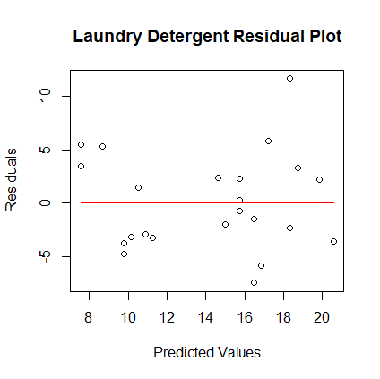
Interpret the residual plot.

Create a normal plot of the residuals with the normal line.

> qqnorm(res, main="Normal Plot of Residuals")
> qqline(res, col="red")

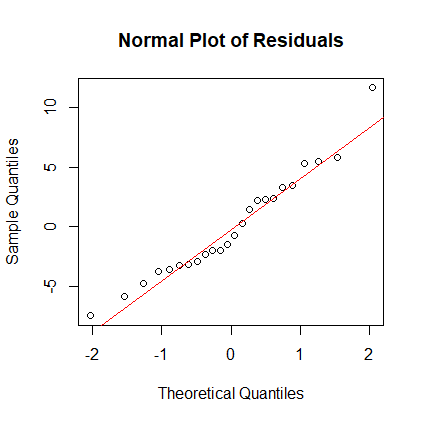
Interpret the normal plot.

With the bears-2024-roster.txt dataset, use R to:

Compute the height in meters and the weight in kilos of the Bears players. The conversion rates are 0.3048 meters per foot and 0.4536 kilos per pound.

> setwd("c:/workspace")
> getwd( )
[1] "c:/workspace"
> bearsDf <- read.csv("bears-2024-roster.txt")
> h <- (bearsDf$HtFt + bearsDf$HtIn / 12) * 0.3048
> h
 [1] 1.8796 1.9050 1.8542 1.9304 1.8542 1.8288 1.9558
 [8] 1.8542 1.8034 1.9304 1.9050 1.9304 1.8288 1.8288
[15] 1.9304 1.9050 1.9812 1.9050 1.9558 1.8796 1.9304
[22] 1.8288 1.9050 1.9304 1.8034 1.8796 1.7526 1.8034
[29] 1.7780 1.9558 1.9812 1.8288 1.8288 1.8542 1.9558
[36] 1.8034 1.8288 1.9304 1.9812 1.8796 1.8288 1.8796
[43] 1.8288 1.8542 1.9304 1.8288 1.8034 1.8288 1.9304
[50] 2.0066 1.9558 1.8796 1.8796 1.7272 1.9050 1.7780
[57] 1.8542 1.9050 1.8288 1.8288 1.8034 1.9812 1.7272
[64] 1.8796 1.9304 1.7526 1.9558
> w <- bearsDf$WtLb * 0.4536
> w
 [1]  95.7096  96.6168 101.6064 136.9872 141.0696 105.6888
 [7] 151.0488  90.7200  96.1632 108.8640 141.0696 139.7088
[13]  92.9880  90.7200 132.4512 136.0800 143.3376 143.3376
[19] 141.5232 134.2656 113.4000 109.7712 111.1320  99.3384
[25]  90.7200 108.8640  96.1632  90.7200  91.6272 145.6056
[31] 100.6992  88.9056  94.3488 102.0600 140.6160  86.1840
[37]  90.7200 121.5648 117.9360 136.0800 102.0600 109.7712
[43]  95.2560  90.7200 139.2552 104.7816  95.2560  88.4520
[49] 136.0800 150.5952 114.7608  91.6272 106.1424  79.3800
[55] 102.5136  83.9160 114.7608 129.2760  93.8952  92.5344
[61]  81.6480 118.8432  97.5240  95.2560 127.0080  81.6480
[67] 151.0488

Find the simple linear regression equation for predicting weight in kilos from height in meters.

> model <- lm(w ~ h)
> model

Call:
lm(formula = w ~ h)

Coefficients:
(Intercept) h 
-331.5 236.0

The linear regression line for predicting weight from height is
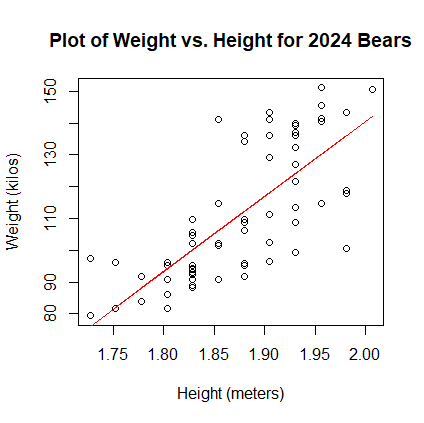
w = 236.0 * h - 331.5

Use R to create a scatter plot of weight (y-axis) vs. height (x-axis). Add the regression line to the plot.

plot(h, w, xlab="Height (meters)", ylab="Weight (kilos)",
+ main="Plot of Weight vs. Height for 2024 Bears")  
> pred <- predict(model)
> lines(h, pred, col="red")

Create the residual plot, which is the residuals (y-axis) vs. the predicted values (x-axis).

> res <- resid(model)
> plot(h, res, xlab="Height (meters)", ylab="Residuals",
+ main="Residual Plot 2024 Bears")
> lines(h, rep(0, length(h)), col="red")

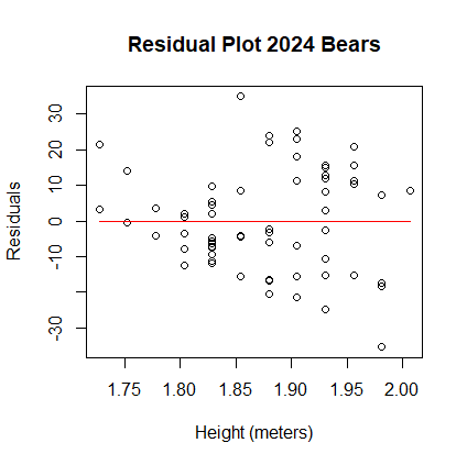
Interpret the residual plot.
Answer: the residuals are slightly biased and heteroscedastic.

Create the normal plot of the residuals. Add the normal line to the plot.

> qqnorm(res, main="Normal Plot of Residuals 2024 Bears")
> qqline(res, col="red")

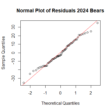
Interpret the normal plot.
Answer: the normal plot shows small random variations above and below the normal line. This means that the residuals are approximately normally distributed.

Project 3

Look at the project description for Project 3 .

The Regression Fallacy

During their flight training, Air Force pilots make two practice landings with their instructor. The pilots that make a good first landing tend to do worse on the second landing; the pilots that make a poor first landing do better on the second landing. Conclusion: criticism helps the pilots, whereas praise hurts them. Policy change: the supervisor of the flight instructors tells them to criticize all landings, good or bad. Is this policy change warrented?
In fact, the criticism is not warrented. This is an example of the regression fallacy.
Look at this graph of pre-test and post-test scores marked by the dots:

The green line indicates where the dots would be if the pre and post scores were the same. The red line is the regression line, which shows where the pre-test score and its associated predicted post-test score would lie. As in the previous example of the Air Force pilots, a student with a high pre-test score is predicted to do worse on the post-test; a student with a low pre-test score is predicted to do better on the post-test.
Practice Problem: Collect the following data for adult men: the subject's height, the height of the subject's father.
1. Would you expect a person with a very tall father to be shorter or taller than his father?
2. Would you expect a person with a very short father to be shorter or taller than his father?

Additional Regression Problem

Root Mean Square Error
A law school finds this relationship between LSAT scores (independent variable x) and first-year scores (dependent variable y). The data are bivariate normal. Here are the summary variables:
x = 162 SD_x = 6
y = 68 SD_y = 10
r = 0.6
1. About what percentage of the students have first-year scores over 75? Because the data are bivariate normal, the first-year scores are normally distributed, so you can use the normal table.
2. Of those students who scored 165 on the LSAT, about what percentage have first-year scores over 75? Visualize these scores as lying in a thin vertical rectangle centered at LSAT = 165.
  Answer: The regression equation is
  y - 68 = (0.6 * 10 / 6) (x - 162)
  y - 68 = 1 (x - 162)
  y = x - 94
  so the predicted value for the students in the thin vertical rectangle centered at x = 165 is y = x - 94 = 165 - 94 = 71.
  
  The RMSE for those students in the thin vertical rectangle centered at x = 165 is
  RMSE = √1 - r² SD_y = √1 - 0.6² 10 = 0.8 * 10 = 8
  
  Then z = (y - y^{^}) / RMSE = (75 - 71) / 8 = 0.5. The area of the bin (-∞, 0.5] is 0.6915 = 69%. Therefore of the students having LSAT score equal to 165, the percentage of students having first year score over 75 is 100% - 69% = 31%.

Obs:	1	2	3	4	5
x:	1	2	3	4	5
y:	1	3	2	5	4