lines <- readLines( )
Ans: The readLines function reads lines from the keyboard. It reads from the Console keyboard like this:
lines <- readLines( )terminate the input with Control-Z for Windows; Control-D for Mac and Unix. For example:
> lines < readLines( )
This
is
a
test.
Control-Z
> lines
[1] "This" "is" "a" "test."
Terminating the keyboard input with Control-Z does not work in RStudio, but you can specify the number of lines to read like this:
> lines <- readLines(n=2)
This
is
>
Ther readLines function also reads from a file:
lines <- readLines("kids.txt")
kids <- read.table("kids.txt", header=F)
Ans: The header is treated as data and the default variables V1, V2, V3, etc. are used
for the columns. You can add column names like this:
kids <- read.table("kids.txt", header=F,
  col.names=c("Age", "Gender", "Age"))
> v <- c(2, 4, 3, 4, 2, 3, 2, 3)
> table(v)  # Show frequency of outcomes in v.
v
2 3 4
3 3 2
> w <- c(1, 3, 1, 1, 3, 3, 1, 1)
>             # Show 3x2 contingency table of
> table(v, w) # outcomes of v and w.
   w
v   1 3
  2 2 1
  3 2 1
  4 1 1
> # Higher dimensional contingency tables are possible.
values <- factor(c(7, 3, 9, 2))
df <- data.frame(n=1:4, a=values)
plot(df)
What is wrong?
Ans: Factors are stored as numeric values. "7", "3", "9", "2" are stored as 3, 2, 4, 1, which are the values that are plotted. This is how to actually plot the character values:
plot(df[ ,1], as.character(df[ ,2]))Of course if the values 7, 3, 9, 2 were entered in column 2 of the data frame instead, these values would not be stored as factors, so the dataframe could be plotted as
plot(df[ ,1], df[ ,2])or, even easier,
plot(df)
Ans: The multinormal distribution occurs frequently in nature. It is also the theoretical basis for linear and quadratic discriminant analysis, which is an important supervised machine learning technique. Perform discriminant analysis in SAS with proc discrim and in R with the lda (linear discriminant analysis) and qda (quadratic discriminant analysis) functions in the MASS package.
Ans: An S3 class is a list with a class attribute that contains the name of the class. To create an S3 object, create a list with the object's data fields, then set the class attribute to the name of the class. An S3 object is usually created with a constructor. Here is the Kid constructor:
kid <- function(theName, theGender, theAge) {
   theObject <- list(name=theName,
      gender=theGender, age=theAge)
   class(theObject) = "Kid"
   return(theObject)
}
Ans: The generic funtion haveBirthday is defined like this:
haveBirthday <- function(theObject) {
   UseMethod("haveBirthday", theObject)
}
This generic function determines the class of the object that is calling it and then calls the
specific haveBirthday method for that class, in this case
haveBirthday.Kid.
v <- c(45, 31, 19, 76, 111)using methods 1 and 4. Verify your results by hand.
Ans: First sort the vector:
19 21 45 76 111Compute the 0.67 quartile = Q(0.67) using Method 1:
We have
| Index: | 1 | 2 | 3 | 4 | 5 |
| Quantile: | 0.2 | 0.4 | 0.6 | 0.8 | 1.0 |
| Value: | x1=19 | x2=21 | x3=45 | x4=76 | x5=111 |
To find the 0.67 quartile, note that 0.67 is between quantile 0.6 and 0.8 in the table--we round up to 0.8, so Q(0.67) = x4 = 76.
Compute Q(0.67) using Method 4:
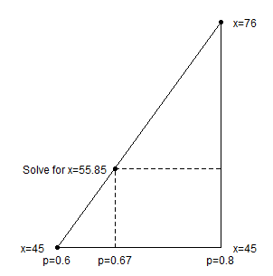
Using the table above we see that Q(0.6) = x3 = 45 and Q(0.8) = x4 = 76. Use linear interpolation to find Q(0.67)

We use similar triangles:
-
(x - 45) / (76 - 45) = (0.67 - 0.6) / (0.8 - 0.6)
(x - 45) / 31 = 0.07 / 0.2
x = 31 * 0.07 / 0.2 + 45 = 55.85
Check with R:
> quantile(v, 0.67, type=1)
67%
76
> quantile(v, 0.67, type=4)
67%
55.85
>
Here is the R script that draws the interpolation diagram.
See the Quantile Computations document for the details of computing quantiles of types 1 to 9.
# Compute quantile using R type 4 calculation.
myQuantileType4(data, p) {
  data <- sort(data)
  n <- length(data)
  j <- floor(p * n)
  pdiff_big = 1 / n
  xdiff_big = data[j + 1] - data[j]
  pdiff_small = p - j / n;
  xdiff_small = xdiff_big * pdiff_small / pdiff_big;
  return(data[j] + xdiff_small)
}

x <- c(19, 21, 45, 76, 111)
myQuantileType4(x, 0.67)
quantile(x, 0.67, type=4)
| R | SAS | |||
|---|---|---|---|---|
| Normal | Uniform | Normal | Uniform | |
| Density (PDF) | dnorm | dunif | pdf("normal", ...) | pdf("uniform", ...) |
| Cumulative (CDF) | pnorm | punif | cdf("normal", ...) | cdf("uniform", ...) |
| Quantile (IDF) | qnorm | qunif | quantile("normal", ...) | quantile("uniform", ...) |
| Random Variable (RV) | rnorm | runif | rand("normal", ...) | rand("uniform", ...) |


