To Documents
Brief SPSS Tutorial
Table of Contents
- Introduction
- Starting Up SPSS
- Entering a New Dataset Manually
- Importing an Excel Dataset
- Transform Variables
- Subsetting a Dataset
- Printing a New Dataset
- Sorting a Dataset
- Descriptive Statistics
- Quartiles and Plots
- Histograms
- Crosstabs Tables
- Normal Plots
- Correlations
- Scatterplots
- Regression Lines and Residual Plots
- One-sample t-tests
- Paired-sample t-tests
- Independent two-sample t-tests
1. Introduction
- SPSS (Statistics Package for the Social Sciences) is a software package
used for conducting statistical analyses, manipulating data, and
generating tables and graphs that summarize data.
Statistical analyses include basic descriptive statistics,
such as averages and frequencies, to advanced inferential
statistics, such as regression, analysis of variance,
and factor analysis.
- SPSS for Windows consists of five different windows, each of which
is associated with a particular SPSS file type. We will examine
two of these windows: the Data Editor and the Output Viewer.
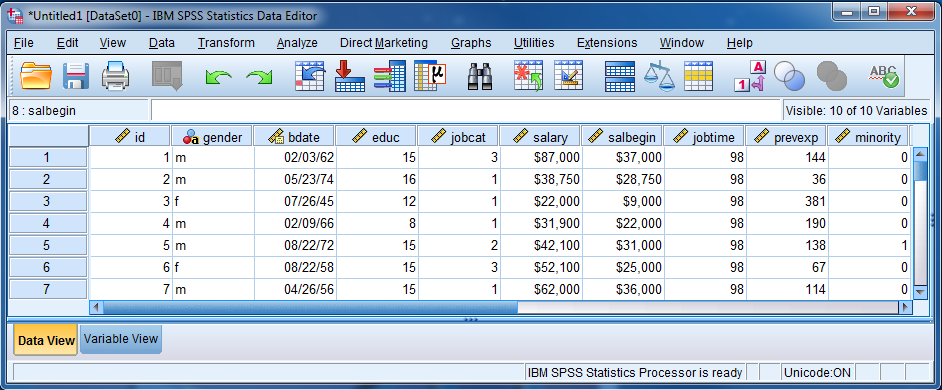
- The Data Editor window displays the contents of the working dataset.
It is arranged in a spreadsheet format that contains variables in
columns and cases in rows. Notice how there are two tabs at the
bottom of the window: Data View, and Variable View.

- The Data View tab lets you examine the data, much like it appears in an Excel
spreadsheet. The Variable View tab allows you to examine information about the
dataset that is stored with the dataset.
- The Output Window shows the results of requested statistical analyses or
graphs. The items in the Output Window can be exported to a Word file
to submit for activities.
2. Starting Up SPSS
- To start up SPSS:
- Click the Start Button, then select All Programs >> Mathematics and Statistics >> IBM SPSS Statistics >> IBM Statistics SPSS 24. SPSS might take up to one minute to load.
- Close the IBM SPSS 24 dialog that tells you what's new.
- This puts you in a SPSS Data Editor Window. To rename the dataset:
- Select the main menu entry File >> Rename Dataset.
- Enter the new dataset name, say Persons1, for the Dataset Name
in the Rename Dataset dialog.
You should see Untitled1 [Persons1] ... in the title bar of the
Data Editor Window.
3. Entering a New Dataset Manually
- To enter a new dataset manually:
- Select the Variable View Tab .
- For each variable in your new dataset specify its characteristics:
- Enter the variable name in the Name column.
- Enter the type (Numeric or String) in the Type column.
- Set the maximum width in characters or digits if you wish in the Width column.
- For any Numeric variables, specify how many digits after
the decimal point you wish to display in the Decimals Column.
- Optional: supply a descriptive label for the variable.
For example, the variable Height might have the label
"Height in Meters".
- Also specify the Measure for each variable. The
choices are Nominal (Categorical), Ordinal and Scale (Continuous).
- Select the Data View Tab at the bottom of the Data Editor Window. Type in
the values of the variables as you would do in an Excel Spreadsheet.
4. Importing an Excel Dataset
- To import an Excel dataset:
- Place the Excel datafile on the harddrive of the machine running SPSS
(Lab computer or studentrds server).
- In the main menu, select File >> Open >> Data. In the Open Data dialog,
select Excel (*.xls) in the Files of type drop down box.
- Select the Excel file to import from the hard drive.
- In the Opening Excel Data Source window, select the worksheet that
you want to import, whether the first row contains the variable name.
- The data can be edited using the data editor after it has been imported.
In the Variable View, you can set the Measure and other dataset variable properties.
5. Transform Variables
- To create a new variable calculated from existing variables:
- Select main menu Transform >> Compute Variable.
- Enter the name of the new variable to be calculated in the
Target Variable textbox.
- Enter the expression for calculating the new variable in
the Numeric Expression textbox. The expression should contain only
operators, numbers and previously defined variables.
- Click the OK button.
- The newly computed variable will appear as a new column in the Data Editor.
6. Subsetting a Dataset
- There are two ways to select only a subset of the current dataset:
- In the main menu, select Data >> Select Cases. Check the radio button
with the caption: "If condition is satisfied". Click the If... Button.
Then in the box at the upper right, enter an expression which rows to keep.
Click OK. Here are two examples:
- x ~= 13 & x ~= 97
- $CaseNum ~= 4 & $CaseNum ~=46
The first example keeps all observations where x is not equal to 13 and
x is not equal to 97. The second example keeps all observations except the
ones with case number equal to 4 and 46.
- Use another column to enter 1s and 0s. A 1 in a row means "keep that row." A
0 in a row means "remove that row." Change the name of the column to filter1 in
the Variable View. Then select Data >> Select Cases.
Check the "Use Filter" button and click on the right arrow to move the
variable named filter1 to the box. Finally click OK.
There should be a diagonal line through each removed observation.
7. Printing a Dataset
- To print the current dataset:
- In the main menu, select Analyze >> Reports >> Case Summaries.
Move the variables you want to print to the Variables Box. Click OK.
8. Sorting a Dataset
- To sort the rows of a dataset by the values in a column:
- In the main menu, select Data >> Sort Cases.
- Move the variable or variables by which you want to sort into the
Sort by Box. Click OK.
The rows in the dataset will now be sorted.
9. Descriptive Statistics
- To compute descriptive statistics such as the mean, standard deviation,
minimum and maximum:
- Go to the Data Editor Window.
- In the main menu, select Analyze >> Descriptive Statistics >>
Descriptives.
- In the Descriptives dialog, move all the variables for which you
want descriptive statistics from the left to the variables box.
- Click on the Options button and select, in the Descriptives: Options
dialog, all the descriptive statistics that you want shown in the output.
Click Continue. The values of the descriptive statistics will
be shown in the Output Window.
10. Quartiles and Plots
- To obtain quartiles (Q0, Q1, Q2, Q3, and Q4):
- Go to the Data Editor Window.
- In the main menu, select Analyze >> Descriptive Statistics >> Explore.
- In the Explore dialog, move all the variables that you want to analyze
to the Dependent List box.
- Click on the Statistics button. In the Explore: Statistics dialog,
check only the boxes Outliers and Percentiles. Click Continue.
- Click on the Plots button. In the Explore: Plots dialog,
check the radio button Dependents together.
Also, check the Stem-and-leaf and Histogram check boxes.
- Click Continue.
- Click the OK button.
- The requested analyses and plots will appear in the output window.
- Here are the statistics that you can obtain using Analyze >> Descriptive
Statistics >> Explore:
-
Count (n), mean (x, standard deviation
(SD+), variance, standard error for the mean
(SEave), 95% confidence interval for the mean,
range, Q0, Q1, Q2, Q3, Q4, IQR, skewness, kurtosis, M-estimators
(Huber's, Tukey's biweight, Hample's, Andrews'),
5, 10, 25, 50, 75, 90, 95 percentiles, extreme values
11. Histograms
- There are three ways to create a histogram:
Method 1:
- In the main menu of the Data Editor Window, select Graphs >> Legacy
Dialogs >> Interactive >> Histogram.
- In the Create Histogram dialog, drag the variable for which you
want to create the histogram into the box marked by the horizontal
arrow. (The box marked by the vertical arrow should contain the
variable Count($count)). A hand icon will appear when the box is ready
to accept the variable you are dragging.
- Set any other options you want to set on the Histogram, Titles
or Options tabs. Click OK on the Create Histogram dialog.
Note, only scale variables can be used for the horizontal variable
of a histogram. If necessary, go to the Variable view in the Data
Editor and change the Measure of the variable on the right to scale.
Method 2:
- Main menu Analyze >> Descriptives >> Explore. Move the variable(s)
that you want to use for your histogram into the Dependent List box.
Click the Plots button and check Histogram. Click OK.
- Usually you will use Method 2 when you want to obtain other graphs
and analyses at the same time, for example, boxplot, stemplot, mean, SD, and
quartiles.
Method 3:
- Select Graphs >> Chartbuilder. Click OK on the Chart Builder dialog.
- Select Histogram from the Choose From: list. Drag a Simple Histogram
into the Chart Preview Area at the upper right.
- Drag the desired variable into the X-Axis? area.
- Go to the Element Properties window and click on the Set Parameters
button.
- Choose the number of bins by selecting the Custom button and
entering the Number of Intervals.
- Click Continue, click Apply, and click OK.
12. Crosstabs Tables
- To create a crosstabs table:
- In the main menu of the Data Editor Window, select Analyze >> Descriptive
Statistics >> Crosstabs.
- In the Crosstabs dialog, move the variables that
you want to use for Rows and for Columns into the
corresponding box. Click OK.
The crosstabs table will appear in the Output Window.
13. Normal Plots
- To create a normal plot:
- Select Analyze >> Descriptive Statistics >> Q-Q Plots. Move the
desired variable to the variables box and select Van der Waerden's as
the Proportion Estimation Formula. Click OK.
A normal plot will be created, which is a plot of the expected normal scores
vs. the actual data points.
14. Correlations
- To compute the pairwise correlations of a set of variables:
- Select main menu Analyze >> Correlate >> Bivariate.
- In the Bivarate Correlations dialog, move all variables for which
you want correlations into the Variables box. Leave the Pearson,
Two-tailed, and Flag significant correlations boxes checked. Click OK.
A matrix will appear in the Output Window that shows the correlation
for each pair of variables. Significant correlations will be marked
with **.
15. Scatterplots and Regression Lines
- To create a scatterplot for a given x- and y-variable,
- Select Graphs >> Chartbuilder. Click OK on the Chart Builder dialog.
- Select Scatter/Dot from the Choose From: list. Drag a Simple Scatterplot
into the Chart Preview Area at the upper right.
- Drag the desired variables into the X-Axis? and Y-Axis? areas.
- Modify any other properties of the graph as desired.
- Click Continue, click Apply, and click OK.
16. Regression Models and Residual Plots
- To obtain the regression equation, while saving the predicted values
and residuals:
- Select Analyze >> Regression >> Linear. Move the desired y-variable
to the Dependent box and the x-variable to the Independent box.
- Click the Stastistics button. Leave the Estimates and Model Fit boxes
checked. Click Continue.
- Don't click the Plots button. The names of the plot types are
confusing. It is better to use the Save button to save
the residuals and predicted values for a scatterplot later.
- Click the Save button. Chick Unstandardized in the Predicted Values
box and Unstandardized in the Residuals box. Click Continue. Click OK.
The regression equation with the R-squared values is displayed in the output.
Two new variables should be created in the dataset: PRE_1 with label
Unstandardized Predicted Values and RES_1 with label Unstandardized
Residuals.
- Create a scatterplot of RES_1 vs. PRE_1.
17. One-sample t-tests
- To perform a one-sample t-test, the response variable values should be
loaded into the Data Editor. Suppose that the response variable name is x.
- Select Analyze >> Compare Means >> One-Sample T Test.
- Move the variable x into the Test Variable(s) box.
- Enter the μ of the null hypothesis.
- Click Options. Select 95 as the confidence interval percentage.
- Click Continue; click OK.
The following information will be recorded in the Output Window:
t-statistic, df (degrees of freedom), Sig.(2-tailed), which is the
p-value, mean difference, confidence interval.
18. Paired-sample t-tests
- To perform a paired-sample t-test, the two response variable values should
be loaded into the Data Editor. Suppose that the response variable names are x and y.
- Select Analyze >> Compare Means >> Paired-Samples T-Test.
- Move the x and y variables into the Paired Variables box.
You will have to select both paired variables before moving them.
- Click Options. Set 95 as the confidence interval percentage.
- Click Continue; click OK.
The following information will be recorded in the Output Window:
descriptive statistics for x and y: n, mean, SD, SE(mean), correlation,
statistics for the difference: mean, SD, SE(mean), 95% confidence interval,
degrees of freedom, sig. (2-tailed), which is the p-value.
19. Independent Two-sample t-tests
- To perform an independent two-sample t-test, the response variable values
should be loaded into a single column x. A second column should contain
the group names. This second column should be a nominal variable, say with
the variable name Group.
- Select Analyze >> Compare Means >> Independent-Samples T-Test.
- Move x to the Test Variable(s) box.
- Move Group to the Grouping Variable box.
- Click the Define Groups button; enter the value for Group 1 and the
value for Group 2. Click Continue.
- Click Options. Set 95 as the confidence interval percentage.
- Click Continue; click OK.
The following information will be recorded in the Output Window:
descriptive statistics for x, computed separately by value of Group,
various statistics used to perform the independent-sample t-test.
The important ones are in the Sig. (2-tailed) column, which give the
p-values. Use the larger p-value to be safe.

