To Notes

Estimates of the Center

The Sample Mean

• The sample mean x is defined as
   
       x = (x₁ + ... + x_n) / n
• For a dataset that has a bell-shaped histogram, the average is the most efficient estimate of the center of the histogram.
• However, for a dataset that has a skewed histogram (for example with a long right tail):
       x is pulled in the direction of the long tail, so Q2 better represents the center of the histogram.
       x is more influenced by outliers than Q2 is.
• Q2 is also a better estimate of the histogram center if the histogram has thick tails (has outliers on both sides).

The Median

• If a histogram is skewed, the median (Q2) is a better estimate of the "center" of the histogram than the sample mean.

Other Measures of Central Tendency

• A third another statistic that has been proposed (in addition to the mean and median) to estimate the center of a dataset: the 5%-trimmed mean: throw out the bottom 2.5% and top 2.5% of the observations, then compute the sample mean of the remaining observations.
• The median and the 5%-trimmed mean are resistant or robust statistics because they are resistant to outliers.
• Resistant to outliers means that the value of the trimmed mean is not affected very much by outliers.
• If there are less than 2.5% outliers on the left and less than 2.5% outliers on the right, then the trimmed mean is more efficient for estimating the center of the histogram than the mean or the median.
• A family of more esoteric statistics to estimate the center of a dataset are the M-estimators. They are weighted averages, which give heavier weight to the observations close to the median and less weight to the observations in the tails.
• To obtain M-estimators with SPSS, select
   
  Analyze >> Descriptive Statistics >> Explore...
   
  Click the Statistics button and check the M-estimators box.
• An M-estimator is a weighted average of the observations, where the weights are chosen to have good theoretical properties.

Bell-shaped Histograms

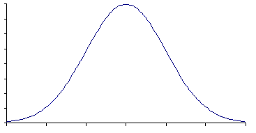
• Many histograms of real data are bell shaped. Here is the standard bell-shaped curve:
   
  
   
       The bell-shaped curve is symmetric around its center.
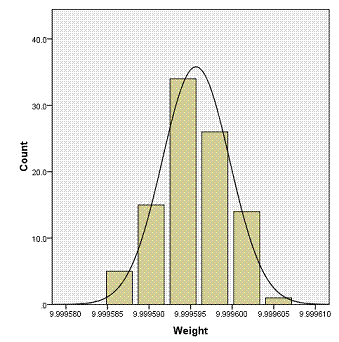
       If we disregard the two extreme outliers, the histogram of the NBS-10 data is roughly bell-shaped.
   
  
• Use SPSS to do the following with the NBS-10 data nbs-10.xls:
  
  1. Find the dataset mean.
  2. Graph the histogram and the boxplot.
  3. Delete the outliers according to the boxplot.
  4. Plot a histogram with superimposed normal curve.
• If a histogram is bell shaped, it can be parsimoniously described by its center and spread.
      The center is the location of its axis of symmetry.
      The spread is the distance between the center and one of its inflection points.
• Here is an a bell-shaped histogram with its inflection points marked.
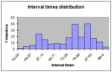
• Here is the histogram of some times between eruptions of the Old Faithful Geyser in minutes:
   
  
• This histogram is not bell-shaped, so the center and spread are not a good summary of the data.
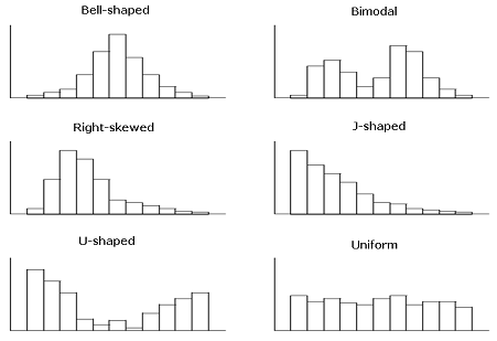
• Here are some histograms and the terms used to describe them:
   
  
• The right-skewed and J-shaped histograms have long right tails.