June 3, 2024

IT 223 -- June 5, 2024

Review Exercises

What are the five steps for executing a z- or t-test?
How does a t-test differ from a z-test?

Degrees of Freedom

Degrees of Freedom (df) is a technical term that arises when using the t-test. We are using x to estimate μ in SD+. If we are computing the SD+, when we are computing the square of the deviations, once we know the first n - 1 deviations, we automatically know the nth deviation because the sum of the deviations is always zero. n - 1 is called the degrees of freedom because only n - 1 of the deviations are able to vary freely.
The degrees of freedom for the t-test is related to the n - 1 that is used in the denominator of SD+.
Taking df = n - 1 compensates for the additional variation introduced because the true mean μ is unknown and x is used to estimate it.

The Paired Sample t-test

Goal: to test whether there is a significant difference between subjects from two different groups.
Typically, one group is the treatment group and the other group is the control group.
To use the paired sample t-test, each subject in one group is matched with a subject in the other group. This reduces the random error in the dataset.
Then compute the differences in the response variable and perform a one-sample t-test on the differences.

Example 7: To test whether a new type of shoe sole material (type B) is better than the old type (type A), manufacture 10 pair of shoes where one shoe is made of type A and the other of type B. Randomly assign the type of material to left or right. Here is the data:

SoleMaterialA	SoleMaterialB
13.2	14.0
8.2	8.8
10.9	11.2
14.3	14.2
10.7	11.8
6.6	6.4
9.5	9.8
10.8	11.3
8.8	9.3
13.3	13.6

Perform the paired-sample t-test to see if there is a real difference between the two sole materials, or if it is just chance variation.

Use R to create a dataframe from this t-test2.txt:

> setwd("c:/it223/sole-material")
> df <- read.csv("t-test2.txt")
> diff <- df$A - df$B
> t.test(diff, mu=0)

         One Sample t-test

data: diff
t = -3.3489, df = 9, p-value = 0.008539
alternative hypothesis: true mean is not equal to 0
95 percent confidence interval:
 -0.6869539 -0.1330461
sample estimates:
mean of x 
     -0.41

Here are the five steps of the two-sample t-test:
1. Write down the null and alternative hypothesis:
  H₀: SoleMaterial A = SoleMaterial B
  H₁: SoleMaterial A ≠ SoleMaterial B
2. Obtain the test statistic from R: t = -3.349
3. Using the t-table, obtain a 95% confidence interval with n - 1 = 10 - 1 = 9 degrees of freedom:
  I = [-2.26, 2.26]
4. t ∉ I so reject H₀.
5. Find the p-value from the R output: p = 0.009.
The test statistic for the two-sample t-test obtained by computing the differences
diff = SolematerialA - SoleMaterialB,
then use R to perform a one-sample t-test on the variable diff.
Here are the five steps of the one-sample t-test performed with the diff variable:
1. Write down the null and alternative hypothesis:
  H₀: diff = 0
  H₁: diff ≠ 0
2. Obtain the test statistic from R: t = -3.349
3. Using the t-table, obtain a 95% confidence interval with n - 1 = 10 - 1 = 9 degrees of freedom:
  I = [-2.26, 2.26]
4. t ∉ I so reject H₀.
5. Find the p-value from the R output:
  p = 0.009.

Simple Linear Regression Example

Example 2: the blood alchohol level for a random sample of college students is tested after they drink a few beers. The data file beer-bac.txt contains two columns: (a) the number of beers (beers) consumed and (b) their blood alchohol levels (bac) after they drink the beers. Analyze the regression model and graphs of the resulting data. Use the output and graphs produced from this R script: beer-bac.R

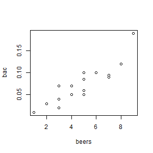
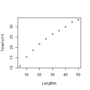
Create the scatter plot of bac vs. beers.

> setwd("c:/it223/beer-bac")
> df1 <- read.csv("beer-bac.txt")
> print(df1)
   beers   bac
1      5 0.100
2      2 0.030
3      9 0.190
4      8 0.120
5      3 0.040
6      7 0.095
7      3 0.070
8      5 0.060
9      3 0.020
10     5 0.050
11     4 0.070
12     6 0.100
13     5 0.085
14     7 0.090
15     1 0.010
16     4 0.050

Scatterplot of original beer-bac data:
Plot of bac vs. beers

Find the linear regression equation for predicting bac from beers:

> model1 <- lm(bac ~ beers, data=df1)
> print(model1)

Call:
lm(formula = bac ~ beers, data = df1)

Coefficients:
(Intercept) beers 
-0.01270 0.01796 

> print(summary(model1))

Call:
lm(formula = bac ~ beers, data = df1)

Residuals:
      Min        1Q    Median        3Q       Max 
-0.027118 -0.017350  0.001773  0.008623  0.041027 

Coefficients:
             Estimate Std. Error t value Pr(>|t|)    
(Intercept) -0.012701   0.012638  -1.005    0.332    
beers        0.017964   0.002402   7.480 2.97e-06 ***
---
Signif. codes:  0 ‘***’ 0.001 ‘**’ 0.01 ‘*’ 0.05 ‘.’ 0.1 ‘ ’ 1

Residual standard error: 0.02044 on 14 degrees of freedom
Multiple R-squared:  0.7998,    Adjusted R-squared:  0.7855 
F-statistic: 55.94 on 1 and 14 DF,  p-value: 2.969e-06

Find the R-squared value for this equation. Interpret it.
Answer: The r-squared value is 0.7998, which is the proportion of the variation in the dependent variable due to the variation of the independent variable. This is a good value for chemistry/biology data.

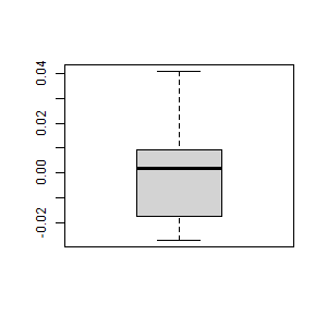
Create the boxplot of the residuals:

> residuals <- resid(model1)
> boxplot(residuals)

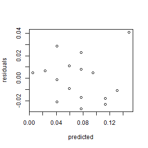
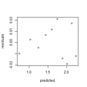
Create the scatterplot of the residuals vs. the predicted values. Interpret it.
```
> predicted <- predict(df1)
> residuals <- resid(df1)
> plot(predicted, residuals)
```
The residuals are unbiased and homoscedastic.
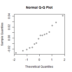
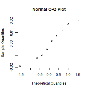
Create the normal plot of the residuals. Interpret it.

The residuals are approximately normally distributed.
For the regression studied in this example, if the number of beers consumed is 4, what is the predicted blood alcohol level?

The Pendulum Data

Perform the pendulum experiment in groups of three.
Take a pendulum consisting of a nut, thread, and paper that indicates the length of the pendulum in inches. Measure the time in seconds that it takes the pendulum to complete 15 complete periods.
Use your phone stopwatch to measure the time for 15 periods. Alternatively, you can use this online stopwatch:
www.online-stopwatch.com/
Record your time to the nearest hundredth of a second.
Here is the pendulum data collected on Monday: pendulum.txt. The fields are LengthIn (length of pendulum in inches) and TimeFor15 (time for 15 periods of the pendulum). Here is the R analysis:
1. Read the raw data from the input file:
```
> setwd("c:/it223/pendulum")
> df1 = read.csv("pendulum.txt")
> print(df1)
  LengthIn TimeFor15
1        5     10.87
2       10     15.42
3       15     18.66
4       20     21.65
5       25     24.21
6       30     26.60
7       35     28.14
8       40     29.99
9       45     32.34
10      50     33.61
```
2. Plot the raw dataset:
```
 > plot(df1)
```
  Plot of df1: original dataset
3. Convert the new data vectors square root of length of pendulum in meters (slen) and time for one pendulum period in seconds (per):
```
> slen <- sqrt(df1$LengthIn * 2.54 / 100)
> print(slen)
[1] 0.3563706 0.5039841 0.6172520 0.7127412 
[5] 0.7968689 0.8729261 0.9428680 1.0079683
[9] 1.0691118 1.1269428
> per <- df1$TimeFor15 / 15
> print(per)
[1] 0.7246667 1.0280000 1.2440000 1.4433333 
[5] 1.6140000 1.7733333 1.8760000 1.9993333 
[9] 2.1560000 2.2406667
```
  Plot of per vs. slen: plot of transformed data:
4. Obtain the regression model for predicting slen from per:
```
> model1 <- lm(per ~ slen)
Call:
lm(formula = per ~ slen)

Coefficients:
(Intercept) slen 
0.03227 1.97034

> summary(model1)

Call:
lm(formula = per ~ slen)

Residuals:
       Min         1Q     Median         3Q        Max 
-0.0189833 -0.0114976 -0.0008825  0.0103954  0.0210963 

Coefficients:
            Estimate Std. Error t value Pr(>|t|)    
(Intercept)  0.03227    0.01631   1.979   0.0832 .  
slen         1.97034    0.01951 100.975 1.03e-13 ***
---
Signif. codes:  0 ‘***’ 0.001 ‘**’ 0.01 ‘*’ 0.05 ‘.’ 0.1 ‘ ’ 1

Residual standard error: 0.01478 on 8 degrees of freedom
Multiple R-squared:  0.9992,    Adjusted R-squared:  0.9991 
F-statistic: 1.02e+04 on 1 and 8 DF,  p-value: 1.033e-13
```
5. Create and interpret the residual and normal plots:
  Residual plot from per ~ slen model:
```
plot(predicted, residuals)
```
  Interpretation of residual plot. The residuals are approximately unbiased and homoscedastic.
6. Normal plot of residuals from per ~ slen model:
```
> qqnorm(residuals)
```
  Interpretation of normal plot: the residuals have slightly thin tails.
7. The theoretical formula for predicting the period of a pendulum from its length is
  per = 2π√len / g = (2π/√g) * √len + 0.0
  where g is the acceleration of gravity. In general g depends on the altitute and the latitude, but g for Chicago is approximately 9.803 m / sec² This means that the true value of the slope is
  2π/√g = 2.006783
  The true value of the intercept is 0.0
8. Find a 95% confidence interval for the slope a. Look up a 95% = 0.025 level confidence interval for the t-statistic. Note that the degrees of freedom are 8: we have 10 observations, but lose one degree of freedom for each parameter (a and b) that is estimated. A 95% confidence interval for 8 degrees of freedom is
  [-2.316, 2.316]. Continuing the computation:
  -2.316 ≤ z ≤ 2.316
  -2.316 ≤ (a^{^} - a) / SE_a^{^} ≤ 2.316
  -2.316 ≤ (1.97034 - a) / 0.01951 ≤ 2.316
  -2.316 * 0.01951 ≤ (1.97034 - a) ≤ 2.316 * 0.01951
  -2.316 * 0.01951 - 1.97034 ≤ -a ≤ 2.316 * 0.01951 - 1.97034
  -2.015525 ≤ -a ≤ -1.925155
  1.925155 ≤ a ≤ 2.015525
  This means that a 95% confidence interval for the true value of a is[1.93, 2.02].
  The true value of a is 2.007, which does belong to the confidence interval.
9. Find a 95% confidence interval for the intercept. Look up a 95% = 0.025 level confidence interval for the t-statistic. Note that the degrees of freedom are 8: we have 10 observations, but lose one degree of freedom for each parameter (a and b) that is estimated. A 95% confidence interval for 8 degrees of freedom is [-2.316, 2.316]. Continuing the computation:
  -2.316 ≤ z ≤ 2.316
  -2.316 ≤ (b^{^} - b) / SE_b^{^} ≤ 2.316
  -2.316 ≤ (0.03227 - b) / 0.01631 ≤ 2.316
  -2.316 * 0.01631 ≤ (0.03227 - b) ≤ 2.316 * 0.01631
  -2.316 * 0.01631 - 0.03227 ≤ -b ≤ 2.316 * 0.01631 - 0.03227
  -0.07004396 ≤ -b ≤ 0.00550396
  -0.00550396 ≤ b ≤ 0.07004396
  THis means that a 95% confidence interval for the true value of b is
  [-0.00553, 0.07004].
  The true value of b is 0.0, which does b belongs to the confidence interval.
10. Conclusion: our experiment is a success.

Exam Info

Look at the materials on the Exam Info Page.