Practice Exam Problems 1

Final Exam Practice Problems 1

For each question, show your work or give a reason explaining your answer. 4 points for the reason, 1 point for the correct answer.

Roger Cotes was the first to publish a study on
1. how well IQ scores fit the normal distribution.
2. the applications of probability to economics.
3. the theory of errors in astronomy.
4. the uses of statistics in genetics.
Ans: c.
Which of these is another name for categorical variables?
a. Continuous b. Nominal c. Ordinal d. Scale

Ans: b. Nominal means that the data is not numbers. This is the term used in SPSS.
If Q1 = 1,230 and Q3 = 5,238, using the boxplot, the observation at 11,389 is
a. a mild outlier b. an extreme outlier c. below the 75th percentile d. the median

Ans: a. IQR = 4,098. The inner fence to the right is at Q3 + 1.5 * IQR = 11,385. The inner fence to the right is at Q3 + 3.0 * IQR = 17,532. 11,389 is between the inner and outer fences, so it is a mild outlier.
What percentage of IQ scores are over 160, assuming that IQ scores are normally distributed?
a. 0.32% b. 0.032% c. 0.0032% d. 0.00032%

Ans: c: 0.0032%.
For the curve shown below, the points shown in red are
a. asymptotes b. critical points c. inflection points d. outliers

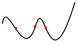
Ans: c: inflection points.
The residual plot that we use in it223 consists of
1. residuals plotted vs. normal scores
2. residuals plotted vs. observation number
3. residuals plotted vs. predicted values
4. y-values plotted vs. x-values
Ans: c. Definition of residual plot.

Show all of your work. You may use a calculator.

Given the following data, draw the box plot.
Q0 = 0.001 Q1 = 0.035 Q2 = 0.057 Q3 = 0.089 Q4 = 0.311
Additional outliers are at 0.141, 0.189, 0.217, 0.240. You decide whether they are mild or extreme.
Compute the correlation of this dataset:
x: 1 2 3 4 5
y: 2 4 7 3 4

Here are the z-scores:
z_x: -1.414 -0.707 0.000 0.707 1.414
z_y: -1.195 0.000 0.000 -0.423 0.000

Ans: r = 0.2536
Here are the summary statistics for the midterm and final scores in a large class:
average midterm score = 50; SD for midterm = 25;

average final score = 55; SD for midterm = 15; r = 0.60

Assume that the data are bivariate normal.
1. About what percentage of students scored over 85 on the midterm?
2. About what percentage of students obtained a score over 85 on the final?
3. Of the students that scored 85 on the midterm, what percentage scored over 85 on the final?
4. Of the students that scored 25 on the midterm, what percentage scored over 85 on the final?

Perform the following analyses with R. Save your output file as a Word .doc file. Type any interpretation of the output into the output file itself.

average midterm score = 50;	SD for midterm = 25;
average final score = 55;	SD for midterm = 15;	r = 0.60